Modelling with ODEs

Ordinary Differential Equations (ODEs) are a powerful tool for modelling a wide range of physical systems. Unlike purely data-driven models, ODEs are based on the underlying physics, biology, or chemistry of the system being modelled. This makes them particularly useful for predicting the behaviour of a system under conditions that have not been observed. In this section, we will introduce the basics of ODE modelling, and illustrate their use with a series of examples written using the DiffSol crate.

The topics covered in this section are:

First Order ODEs: First order ODEs are the simplest type of ODE. Any ODE system can be written as a set of first order ODEs, so libraries like DiffSol are designed such that the user provides their equations in this form.
- Example: Population Dynamics: A simple example of a first order ODE system, modelling the interaction of predator and prey populations.
Higher Order ODEs: Higher order ODEs are equations that involve derivatives of order greater than one. These can be converted to a system of first order ODEs, which is the form that DiffSol expects.
- Example: Spring-mass systems: A simple example of a higher order ODE system, modelling the motion of a damped spring-mass system.
Discrete Events: Discrete events are events that occur at specific times or when the system is in a particular state, rather than continuously. These can be modelled by treating the events as changes in the ODE system's state. DiffSol provides an API to detect and handle these events.
- Example: Compartmental models of Drug Delivery: Pharmacokinetic models describe how a drug is absorbed, distributed, metabolised, and excreted by the body. They are a common example of systems with discrete events, as the drug is often administered at discrete times.
- Example: Bouncing Ball: A simple example of a system where the discrete event occurs when the ball hits the ground, instead of at a specific time.
DAEs via the Mass Matrix: Differential Algebraic Equations (DAEs) are a generalisation of ODEs that include algebraic equations as well as differential equations. DiffSol can solve DAEs by treating them as ODEs with a mass matrix. This section explains how to use the mass matrix to solve DAEs.
- Example: Electrical Circuits: Electrical circuits are a common example of DAEs, here we will model a simple low-pass LRC filter circuit.
PDEs: Partial Differential Equations (PDEs) are a generalisation of ODEs that involve derivatives with respect to more than one variable (e.g. a spatial variable). DiffSol can be used to solver PDEs using the method of lines, where the spatial derivatives are discretised to form a system of ODEs.
- Example: Heat Equation: The heat equation describes how heat diffuses in a domain over time. We will solve the heat equation in a 1D domain with Dirichlet boundary conditions.
- Example: Physics-based Battery Simulation: A more complex example of a PDE system, modelling the charge and discharge of a lithium-ion battery. For this example we will use the PyBaMM library to form the ODE system, and DiffSol to solve it.

Explicit First Order ODEs

Ordinary Differential Equations (ODEs) are often called rate equations because they describe how the rate of change of a system depends on its current state. For example, lets assume we wish to model the growth of a population of cells within a petri dish. We could define the state of the system as the concentration of cells in the dish, and assign this state to a variable $c$. The rate of change of the system would then be the rate at which the concentration of cells changes with time, which we could denote as $\frac{dc}{dt}$. We know that our cells will grow at a rate proportional to the current concentration of cells, so this can be written as:

\[ \frac{dc}{dt} = k c \]

where $k$ is a constant that describes the growth rate of the cells. This is a first order ODE, because it involves only the first derivative of the state variable $c$ with respect to time.

We can extend this further to solve multiple equations simultaineously, in order to model the rate of change of more than one quantity. For example, say we had two populations of cells in the same dish that grow with different rates. We could define the state of the system as the concentrations of the two cell populations, and assign these states to variables $c_1$ and $c_2$. could then write down both equations as:

\[ \begin{align*} \frac{dc_1}{dt} &= k_1 c_1 \\ \frac{dc_2}{dt} &= k_2 c_2 \end{align*} \]

and then combine them in a vector form as:

\[ \begin{bmatrix} \frac{dc_1}{dt} \\ \frac{dc_2}{dt} \end{bmatrix} = \begin{bmatrix} k_1 c_1 \\ k_2 c_2 \end{bmatrix} \]

By defining a new vector of state variables $\mathbf{y} = [c_1, c_2]$ and a vector valued function $\mathbf{f}(\mathbf{y}, t) = \begin{bmatrix} k_1 c_1 \\ k_2 c_2 \end{bmatrix}$, we are left with the standard form of a explicit first order ODE system:

\[ \frac{d\mathbf{y}}{dt} = \mathbf{f}(\mathbf{y}, t) \]

This is an explicit equation for the derivative of the state, $\frac{d\mathbf{y}}{dt}$, as a function of only of the state variables $\mathbf{y}$ and of time $t$.

We need one more piece of information to solve this system of ODEs: the initial conditions for the populations at time $t = 0$. For example, if we started with a concentration of 10 for the first population and 5 for the second population, we would write:

\[ \mathbf{y}(0) = \begin{bmatrix} 10 \\ 5 \end{bmatrix} \]

Many ODE solver libraries, like DiffSol, require users to provide their ODEs in the form of a set of explicit first order ODEs. Given both the system of ODEs and the initial conditions, the solver can then integrate the equations forward in time to find the solution $\mathbf{y}(t)$. This is the general process for solving ODEs, so it is important to know how to translate your problem into a set of first order ODEs, and thus to the general form of a explicit first order ODE system shown above. In the next two sections, we will look at an example of a first order ODE system in the area of population dynamics, and then solve it using DiffSol.

Population Dynamics - Predator-Prey Model

In this example, we will model the population dynamics of a predator-prey system using a set of first order ODEs. The Lotka-Volterra equations are a classic example of a predator-prey model, and describe the interactions between two species in an ecosystem. The first species is a prey species, which we will call $x$, and the second species is a predator species, which we will call $y$.

The rate of change of the prey population is governed by two terms: growth and predation. The growth term represents the natural increase in the prey population in the absence of predators, and is proportional to the current population of prey. The predation term represents the rate at which the predators consume the prey, and is proportional to the product of the prey and predator populations. The rate of change of the prey population can be written as:

\[ \frac{dx}{dt} = a x - b x y \]

where $a$ is the growth rate of the prey population, and $b$ is the predation rate.

The rate of change of the predator population is also governed by two terms: death and growth. The death term represents the natural decrease in the predator population in the absence of prey, and is proportional to the current population of predators. The growth term represents the rate at which the predators reproduce, and is proportional to the product of the prey and predator populations, since the predators need to consume the prey to reproduce. The rate of change of the predator population can be written as:

\[ \frac{dy}{dt} = c x y - d y \]

where $c$ is the reproduction rate of the predators, and $d$ is the death rate.

The Lotka-Volterra equations are a simple model of predator-prey dynamics, and make several assumptions that may not hold in real ecosystems. For example, the model assumes that the prey population grows exponentially in the absence of predators, that the predator population decreases linearly in the absence of prey, and that the spatial distribution of the species has no effect. Despite these simplifications, the Lotka-Volterra equations capture some of the essential features of predator-prey interactions, such as oscillations in the populations and the dependence of each species on the other. When modelling with ODEs, it is important to consider the simplest model that captures the behaviour of interest, and to be aware of the assumptions that underlie the model.

Putting the two equations together, we have a system of two first order ODEs:

\[ \frac{x}{dt} = a x - b x y \\ \frac{y}{dt} = c x y - d y \]

which can be written in vector form as:

\[ \begin{bmatrix} \frac{dx}{dt} \\ \frac{dy}{dt} \end{bmatrix} = \begin{bmatrix} a x - b x y \\ c x y - d y \end{bmatrix} \]

or in the general form of a first order ODE system:

\[ \frac{d\mathbf{y}}{dt} = \mathbf{f}(\mathbf{y}, t) \]

where

\[\mathbf{y} = \begin{bmatrix} x \\ y \end{bmatrix} \]

and

\[\mathbf{f}(\mathbf{y}, t) = \begin{bmatrix} a x - b x y \\ c x y - d y \end{bmatrix}\]

We also have initial conditions for the populations at time $t = 0$. We can set both populations to 1 at the start like so:

\[ \mathbf{y}(0) = \begin{bmatrix} 1 \\ 1 \end{bmatrix} \]

Let's solve this system of ODEs using the DiffSol crate. We will use the DiffSL domain-specific language to specify the problem. We could have also used Rust closures, but this allows us to illustrate the modelling process with a minimum of Rust syntax.

fn main() {
use std::fs;
use diffsol::{
    DiffSl, CraneliftModule, OdeBuilder, OdeSolverMethod
};
use plotly::{
    Plot, Scatter, common::Mode, layout::Layout, layout::Axis
};
type M = nalgebra::DMatrix<f64>;
type LS = diffsol::NalgebraLU<f64>;
type CG = CraneliftModule;
        
let eqn = DiffSl::<M, CG>::compile("
    a { 2.0/3.0 } b { 4.0/3.0 } c { 1.0 } d { 1.0 }
    u_i {
        y1 = 1,
        y2 = 1,
    }
    F_i {
        a * y1 - b * y1 * y2,
        c * y1 * y2 - d * y2,
    }
").unwrap();
let problem = OdeBuilder::<M>::new()
    .build_from_eqn(eqn).unwrap();
let mut solver = problem.bdf::<LS>().unwrap();
let (ys, ts) = solver.solve(40.0).unwrap();

let prey: Vec<_> = ys.row(0).into_iter().copied().collect();
let predator: Vec<_> = ys.row(1).into_iter().copied().collect();
let time: Vec<_> = ts.into_iter().collect();

let prey = Scatter::new(time.clone(), prey).mode(Mode::Lines).name("Prey");
let predator = Scatter::new(time, predator).mode(Mode::Lines).name("Predator");

let mut plot = Plot::new();
plot.add_trace(prey);
plot.add_trace(predator);

let layout = Layout::new()
    .x_axis(Axis::new().title("t"))
    .y_axis(Axis::new().title("population"));
plot.set_layout(layout);
let plot_html = plot.to_inline_html(Some("prey-predator"));
fs::write("../src/primer/images/prey-predator.html", plot_html).expect("Unable to write file");
}

A phase plane plot of the predator-prey system is a useful visualisation of the dynamics of the system. This plot shows the prey population on the x-axis and the predator population on the y-axis. Trajectories in the phase plane represent the evolution of the populations over time. Lets reframe the equations to introduce a new parameter $y_0$ which is the initial predator and prey population. We can then plot the phase plane for different values of $y_0$ to see how the system behaves for different initial conditions.

Our initial conditions are now:

\[ \mathbf{y}(0) = \begin{bmatrix} y_0 \\ y_0 \end{bmatrix} \]

so we can solve this system for different values of $y_0$ and plot the phase plane for each case. We will use similar code as above, but we will introduce our new parameter and loop over different values of $y_0$

fn main() {
use std::fs;
use diffsol::{
    DiffSl, CraneliftModule, OdeBuilder, OdeSolverMethod, OdeEquations
};
use plotly::{
    Plot, Scatter, common::Mode, layout::Layout, layout::Axis
};
type M = nalgebra::DMatrix<f64>;
type LS = diffsol::NalgebraLU<f64>;
type CG = CraneliftModule;
        
let eqn = DiffSl::<M, CG>::compile("
    in = [ y0 ]
    y0 { 1.0 }
    a { 2.0/3.0 } b { 4.0/3.0 } c { 1.0 } d { 1.0 }
    u_i {
        y1 = y0,
        y2 = y0,
    }
    F_i {
        a * y1 - b * y1 * y2,
        c * y1 * y2 - d * y2,
    }
").unwrap();

let mut problem = OdeBuilder::<M>::new().p([1.0]).build_from_eqn(eqn).unwrap();

let mut plot = Plot::new();
for y0 in (1..6).map(f64::from) {
    let p = nalgebra::DVector::from_element(1, y0);
    problem.eqn_mut().set_params(&p);
    
    let mut solver = problem.bdf::<LS>().unwrap();
    let (ys, _ts) = solver.solve(40.0).unwrap();

    let prey: Vec<_> = ys.row(0).into_iter().copied().collect();
    let predator: Vec<_> = ys.row(1).into_iter().copied().collect();

    let phase = Scatter::new(prey, predator)
        .mode(Mode::Lines).name(format!("y0 = {}", y0));
    plot.add_trace(phase);
}

let layout = Layout::new()
    .x_axis(Axis::new().title("x"))
    .y_axis(Axis::new().title("y"));
plot.set_layout(layout);
let plot_html = plot.to_inline_html(Some("prey-predator2"));
fs::write("../src/primer/images/prey-predator2.html", plot_html).expect("Unable to write file");
}

Higher Order ODEs

The order of an ODE is the highest derivative that appears in the equation. So far, we have only looked at first order ODEs, which involve only the first derivative of the state variable with respect to time. However, many physical systems are described by higher order ODEs, which involve second or higher derivatives of the state variable. A simple example of a second order ODE is the motion of a mass under the influence of gravity. The equation of motion for the mass can be written as:

\[ \frac{d^2x}{dt^2} = -g \]

where $x$ is the position of the mass, $t$ is time, and $g$ is the acceleration due to gravity. This is a second order ODE because it involves the second derivative of the position with respect to time.

Higher order ODEs can always be rewritten as a system of first order ODEs by introducing new variables. For example, we can rewrite the second order ODE above as a system of two first order ODEs by introducing a new variable for the velocity of the mass:

\[ \begin{align*} \frac{dx}{dt} &= v \\ \frac{dv}{dt} &= -g \end{align*} \]

where $v = \frac{dx}{dt}$ is the velocity of the mass. This is a system of two first order ODEs, which can be written in vector form as:

\[ \frac{d\mathbf{y}}{dt} = \mathbf{f}(\mathbf{y}, t) \]

where

\[ \mathbf{y} = \begin{bmatrix} x \\ v \end{bmatrix} \]

and

\[ \mathbf{f}(\mathbf{y}, t) = \begin{bmatrix} v \\ -g \end{bmatrix} \]

In the next section, we'll look at another example of a higher order ODE system: the spring-mass system, and solve this using DiffSol.

Example: Spring-mass systems

We will model a damped spring-mass system using a second order ODE. The system consists of a mass $m$ attached to a spring with spring constant $k$, and a damping force proportional to the velocity of the mass with damping coefficient $c$.

The equation of motion for the mass can be written as:

\[ m \frac{d^2x}{dt^2} = -k x - c \frac{dx}{dt} \]

where $x$ is the position of the mass, $t$ is time, and the negative sign on the right hand side indicates that the spring force and damping force act in the opposite direction to the displacement of the mass.

We can convert this to a system of two first order ODEs by introducing a new variable for the velocity of the mass:

\[ \begin{align*} \frac{dx}{dt} &= v \\ \frac{dv}{dt} &= -\frac{k}{m} x - \frac{c}{m} v \end{align*} \]

where $v = \frac{dx}{dt}$ is the velocity of the mass.

We can solve this system of ODEs using DiffSol with the following code:

fn main() {
use std::fs;
use diffsol::{
    DiffSl, CraneliftModule, OdeBuilder, OdeSolverMethod
};
use plotly::{
    Plot, Scatter, common::Mode, layout::Layout, layout::Axis
};
type M = nalgebra::DMatrix<f64>;
type CG = CraneliftModule;
type LS = diffsol::NalgebraLU<f64>;
        
let eqn = DiffSl::<M, CG>::compile("
    k { 1.0 } m { 1.0 } c { 0.1 }
    u_i {
        x = 1,
        v = 0,
    }
    F_i {
        v,
        -k/m * x - c/m * v,
    }
").unwrap();
let problem = OdeBuilder::<M>::new()
    .build_from_eqn(eqn).unwrap();
let mut solver = problem.bdf::<LS>().unwrap();
let (ys, ts) = solver.solve(40.0).unwrap();

let x: Vec<_> = ys.row(0).into_iter().copied().collect();
let time: Vec<_> = ts.into_iter().collect();

let x_line = Scatter::new(time.clone(), x).mode(Mode::Lines);

let mut plot = Plot::new();
plot.add_trace(x_line);

let layout = Layout::new()
    .x_axis(Axis::new().title("t"))
    .y_axis(Axis::new().title("x"));
plot.set_layout(layout);
let plot_html = plot.to_inline_html(Some("sping-mass-system"));
fs::write("../src/primer/images/spring-mass-system.html", plot_html).expect("Unable to write file");
}

Discrete Events

ODEs describe the continuous evolution of a system over time, but many systems also involve discrete events that occur at specific times. For example, in a compartmental model of drug delivery, the administration of a drug is a discrete event that occurs at a specific time. In a bouncing ball model, the collision of the ball with the ground is a discrete event that changes the state of the system. It is normally difficult to model these events using ODEs alone, as they require a different approach to handle the discontinuities in the system. While we can represent discrete events mathematically using delta functions, many ODE solvers are not designed to handle discontinuities, and may produce inaccurate results or fail to converge during the integration.

DiffSol provides a way to model discrete events in a system of ODEs by allowing users to manipulate the internal state of each solver during the time-stepping. Each solver has an internal state that holds information such as the current time $t$, the current state of the system $\mathbf{y}$, and other solver-specific information. When a discrete event occurs, the user can update the internal state of the solver to reflect the change in the system, and then continue the integration of the ODE as normal.

DiffSol also provides a way to stop the integration of the ODEs, either at a specific time or when a specific condition is met. This can be useful for modelling systems with discrete events, as it allows the user to control the integration of the ODEs and to handle the events in a flexible way.

The Solving the Problem and Root Finding sections provides an introduction to the API for solving ODEs and detecting events with DiffSol. In the next two sections, we will look at two examples of systems with discrete events: compartmental models of drug delivery and bouncing ball models, and solve them using DiffSol using this API.

Example: Compartmental models of Drug Delivery

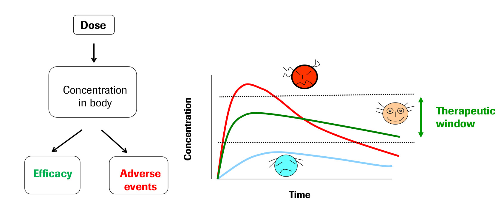
The field of Pharmacokinetics (PK) provides a quantitative basis for describing the delivery of a drug to a patient, the diffusion of that drug through the plasma/body tissue, and the subsequent clearance of the drug from the patient's system. PK is used to ensure that there is sufficient concentration of the drug to maintain the required efficacy of the drug, while ensuring that the concentration levels remain below the toxic threshold. Pharmacokinetic (PK) models are often combined with Pharmacodynamic (PD) models, which model the positive effects of the drug, such as the binding of a drug to the biological target, and/or undesirable side effects, to form a full PKPD model of the drug-body interaction. This example will only focus on PK, neglecting the interaction with a PD model.

Fig 1

PK enables the following processes to be quantified:

Absorption
Distribution
Metabolism
Excretion

These are often referred to as ADME, and taken together describe the drug concentration in the body when medicine is prescribed. These ADME processes are typically described by zeroth-order or first-order rate reactions modelling the dynamics of the quantity of drug $q$, with a given rate parameter $k$, for example:

\[ \frac{dq}{dt} = -k^*, \]

\[ \frac{dq}{dt} = -k q. \]

The body itself is modelled as one or more compartments, each of which is defined as a kinetically homogeneous unit (these compartments do not relate to specific organs in the body, unlike Physiologically based pharmacokinetic, PBPK, modeling). There is typically a main central compartment into which the drug is administered and from which the drug is excreted from the body, combined with zero or more peripheral compartments to which the drug can be distributed to/from the central compartment (See Fig 2). Each peripheral compartment is only connected to the central compartment.

Fig 2

The following example PK model describes the two-compartment model shown diagrammatically in the figure above. The time-dependent variables to be solved are the drug quantity in the central and peripheral compartments, $q_c$ and $q_{p1}$ (units: [ng]) respectively.

\[ \frac{dq_c}{dt} = \text{Dose}(t) - \frac{q_c}{V_c} CL - Q_{p1} \left ( \frac{q_c}{V_c} - \frac{q_{p1}}{V_{p1}} \right ), \]

\[ \frac{dq_{p1}}{dt} = Q_{p1} \left ( \frac{q_c}{V_c} - \frac{q_{p1}}{V_{p1}} \right ). \]

This model describes an intravenous bolus dosing protocol, with a linear clearance from the central compartment (non-linear clearance processes are also possible, but not considered here). The dose function $\text{Dose}(t)$ will consist of instantaneous doses of $X$ ng of the drug at one or more time points. The other input parameters to the model are:

$V_c$ [mL], the volume of the central compartment
$V_{p1}$ [mL], the volume of the first peripheral compartment
$CL$ [mL/h], the clearance/elimination rate from the central compartment
$Q_{p1}$ [mL/h], the transition rate between central compartment and peripheral compartment 1

We will solve this system of ODEs using the DiffSol crate. Rather than trying to write down the dose function as a mathematical function, we will neglect the dose function from the equations and instead using DiffSol's API to specify the dose at specific time points.

First lets write down the equations in the standard form of a first order ODE system:

\[ \frac{d\mathbf{y}}{dt} = \mathbf{f}(\mathbf{y}, t) \]

where

\[ \mathbf{y} = \begin{bmatrix} q_c \\ q_{p1} \end{bmatrix} \]

and

\[ \mathbf{f}(\mathbf{y}, t) = \begin{bmatrix} - \frac{q_c}{V_c} CL - Q_{p1} \left ( \frac{q_c}{V_c} - \frac{q_{p1}}{V_{p1}} \right ) \\ Q_{p1} \left ( \frac{q_c}{V_c} - \frac{q_{p1}}{V_{p1}} \right ) \end{bmatrix} \]

We will also need to specify the initial conditions for the system:

\[ \mathbf{y}(0) = \begin{bmatrix} 0 \\ 0 \end{bmatrix} \]

For the dose function, we will specify a dose of 1000 ng at regular intervals of 6 hours. We will also specify the other parameters of the model:

\[ V_c = 1000 \text{ mL}, \quad V_{p1} = 1000 \text{ mL}, \quad CL = 100 \text{ mL/h}, \quad Q_{p1} = 50 \text{ mL/h} \]

Let's now solve this system of ODEs using DiffSol. To implement the discrete dose events, we set a stop time for the simulation at each dose event using the OdeSolverMethod::set_stop_time method. During timestepping we can check the return value of the OdeSolverMethod::step method to see if the solver has reached the stop time. If it has, we can apply the dose and continue the simulation.

fn main() {
use std::fs;
use diffsol::{
    DiffSl, CraneliftModule, OdeBuilder, OdeSolverMethod, OdeSolverStopReason,
};
use plotly::{
    Plot, Scatter, common::Mode, layout::Layout, layout::Axis
};
type M = nalgebra::DMatrix<f64>;
type CG = CraneliftModule;
type LS = diffsol::NalgebraLU<f64>;
        
let eqn = DiffSl::<M, CG>::compile("
    Vc { 1000.0 } Vp1 { 1000.0 } CL { 100.0 } Qp1 { 50.0 }
    u_i {
        qc = 0,
        qp1 = 0,
    }
    F_i {
        - qc / Vc * CL - Qp1 * (qc / Vc - qp1 / Vp1),
        Qp1 * (qc / Vc - qp1 / Vp1),
    }
").unwrap();

let problem = OdeBuilder::<M>::new().build_from_eqn(eqn).unwrap();
let mut solver = problem.bdf::<LS>().unwrap();
let doses = vec![(0.0, 1000.0), (6.0, 1000.0), (12.0, 1000.0), (18.0, 1000.0)];

let mut q_c = Vec::new();
let mut q_p1 = Vec::new();
let mut time = Vec::new();

// apply the first dose and save the initial state
solver.state_mut().y[0] = doses[0].1;
q_c.push(solver.state().y[0]);
q_p1.push(solver.state().y[1]);
time.push(0.0);

// solve and apply the remaining doses
for (t, dose) in doses.into_iter().skip(1) {
    solver.set_stop_time(t).unwrap();
    loop {
        let ret = solver.step();
        q_c.push(solver.state().y[0]);
        q_p1.push(solver.state().y[1]);
        time.push(solver.state().t);
        match ret {
            Ok(OdeSolverStopReason::InternalTimestep) => continue,
            Ok(OdeSolverStopReason::TstopReached) => break,
            _ => panic!("unexpected solver error"),
        }
    }
    solver.state_mut().y[0] += dose;
}
let mut plot = Plot::new();
let q_c = Scatter::new(time.clone(), q_c).mode(Mode::Lines).name("q_c");
let q_p1 = Scatter::new(time, q_p1).mode(Mode::Lines).name("q_p1");
plot.add_trace(q_c);
plot.add_trace(q_p1);

let layout = Layout::new()
    .x_axis(Axis::new().title("t [h]"))
    .y_axis(Axis::new().title("amount [ng]"));
plot.set_layout(layout);
let plot_html = plot.to_inline_html(Some("drug-delivery"));
fs::write("../src/primer/images/drug-delivery.html", plot_html).expect("Unable to write file");
}

Example: Bouncing Ball

Modelling a bouncing ball is a simple and intuitive example of a system with discrete events. The ball is dropped from a height $h$ and bounces off the ground with a coefficient of restitution $e$. When the ball hits the ground, its velocity is reversed and scaled by the coefficient of restitution, and the ball rises and then continues to fall until it hits the ground again. This process repeats until halted.

The second order ODE that describes the motion of the ball is given by:

\[ \frac{d^2x}{dt^2} = -g \]

where $x$ is the position of the ball, $t$ is time, and $g$ is the acceleration due to gravity. We can rewrite this as a system of two first order ODEs by introducing a new variable for the velocity of the ball:

\[ \begin{align*} \frac{dx}{dt} &= v \\ \frac{dv}{dt} &= -g \end{align*} \]

where $v = \frac{dx}{dt}$ is the velocity of the ball. This is a system of two first order ODEs, which can be written in vector form as:

\[ \frac{d\mathbf{y}}{dt} = \mathbf{f}(\mathbf{y}, t) \]

where

\[ \mathbf{y} = \begin{bmatrix} x \\ v \end{bmatrix} \]

and

\[ \mathbf{f}(\mathbf{y}, t) = \begin{bmatrix} v \\ -g \end{bmatrix} \]

The initial conditions for the ball, including the height from which it is dropped and its initial velocity, are given by:

\[ \mathbf{y}(0) = \begin{bmatrix} h \\ 0 \end{bmatrix} \]

When the ball hits the ground, we need to update the velocity of the ball according to the coefficient of restitution, which is the ratio of the velocity after the bounce to the velocity before the bounce. The velocity after the bounce $v'$ is given by:

\[ v' = -e v \]

where $e$ is the coefficient of restitution. However, to implement this in our ODE solver, we need to detect when the ball hits the ground. We can do this by using DiffSol's event handling feature, which allows us to specify a function that is equal to zero when the event occurs, i.e. when the ball hits the ground. This function $g(\mathbf{y}, t)$ is called an event or root function, and for our bouncing ball problem, it is given by:

\[ g(\mathbf{y}, t) = x \]

where $x$ is the position of the ball. When the ball hits the ground, the event function will be zero and DiffSol will stop the integration, and we can update the velocity of the ball accordingly.

In code, the bouncing ball problem can be solved using DiffSol as follows:

fn main() {
use std::fs;
use diffsol::{
    DiffSl, CraneliftModule, OdeBuilder, OdeSolverMethod, OdeSolverStopReason,
};
use plotly::{
    Plot, Scatter, common::Mode, layout::Layout, layout::Axis
};
type M = nalgebra::DMatrix<f64>;
type CG = CraneliftModule;
type LS = diffsol::NalgebraLU<f64>;
        
let eqn = DiffSl::<M, CG>::compile("
    g { 9.81 } h { 10.0 }
    u_i {
        x = h,
        v = 0,
    }
    F_i {
        v,
        -g,
    }
    stop {
        x,
    }
").unwrap();

let e = 0.8;
let problem = OdeBuilder::<M>::new().build_from_eqn(eqn).unwrap();
let mut solver = problem.bdf::<LS>().unwrap();

let mut x = Vec::new();
let mut v = Vec::new();
let mut t = Vec::new();
let final_time = 10.0;

// save the initial state
x.push(solver.state().y[0]);
v.push(solver.state().y[1]);
t.push(0.0);

// solve until the final time is reached
solver.set_stop_time(final_time).unwrap();
loop {
    match solver.step() {
        Ok(OdeSolverStopReason::InternalTimestep) => (),
        Ok(OdeSolverStopReason::RootFound(t)) => {
            // get the state when the event occurred
            let mut y = solver.interpolate(t).unwrap();

            // update the velocity of the ball
            y[1] *= -e;

            // make sure the ball is above the ground
            y[0] = y[0].max(f64::EPSILON);

            // set the state to the updated state
            solver.state_mut().y.copy_from(&y);
            solver.state_mut().dy[0] = y[1];
            *solver.state_mut().t = t;
        },
        Ok(OdeSolverStopReason::TstopReached) => break,
        Err(_) => panic!("unexpected solver error"),
    }
    x.push(solver.state().y[0]);
    v.push(solver.state().y[1]);
    t.push(solver.state().t);
}
let mut plot = Plot::new();
let x = Scatter::new(t.clone(), x).mode(Mode::Lines).name("x");
let v = Scatter::new(t, v).mode(Mode::Lines).name("v");
plot.add_trace(x);
plot.add_trace(v);

let layout = Layout::new()
    .x_axis(Axis::new().title("t"))
    .y_axis(Axis::new());
plot.set_layout(layout);
let plot_html = plot.to_inline_html(Some("bouncing-ball"));
fs::write("../src/primer/images/bouncing-ball.html", plot_html).expect("Unable to write file");
}

DAEs via the Mass Matrix

Differential-algebraic equations (DAEs) are a generalisation of ordinary differential equations (ODEs) that include algebraic equations, or equations that do not involve derivatives. Algebraic equations can arise in many physical systems and often are used to model constraints on the system, such as conservation laws or other relationships between the state variables. For example, in an electrical circuit, the current flowing into a node must equal the current flowing out of the node, which can be written as an algebraic equation.

DAEs can be written in the general implicit form:

\[ \mathbf{F}(\mathbf{y}, \mathbf{y}', t) = 0 \]

where $\mathbf{y}$ is the vector of state variables, $\mathbf{y}'$ is the vector of derivatives of the state variables, and $\mathbf{F}$ is a vector-valued function that describes the system of equations. However, for the purposes of this primer and the capabilities of DiffSol, we will focus on a specific form of DAEs called index-1 or semi-explicit DAEs, which can be written as a combination of differential and algebraic equations:

\[ \begin{align*} \frac{d\mathbf{y}}{dt} &= \mathbf{f}(\mathbf{y}, t) \\ 0 &= \mathbf{g}(\mathbf{y}, t) \end{align*} \]

where $\mathbf{f}$ is the vector-valued function that describes the differential equations and $\mathbf{g}$ is the vector-valued function that describes the algebraic equations. The key difference between DAEs and ODEs is that DAEs include algebraic equations that must be satisfied at each time step, in addition to the differential equations that describe the rate of change of the state variables.

How does this relate to the standard form of an explicit ODE that we have seen before? Recall that an explicit ODE can be written as:

\[ \frac{d\mathbf{y}}{dt} = \mathbf{f}(\mathbf{y}, t) \]

Lets update this equation to include a matrix $\mathbf{M}$ that multiplies the derivative term:

\[ M \frac{d\mathbf{y}}{dt} = \mathbf{f}(\mathbf{y}, t) \]

When $M$ is the identity matrix (i.e. a matrix with ones along the diagonal), this reduces to the standard form of an explicit ODE. However, when $M$ has diagonal entries that are zero, this introduces algebraic equations into the system and it reduces to the semi-explicit DAE equations show above. The matrix $M$ is called the mass matrix.

Thus, we now have a general form of a set of differential equations, that includes both ODEs and semi-explicit DAEs. This general form is used by DiffSol to allow users to specify a wide range of problems, from simple ODEs to more complex DAEs. In the next section, we will look at a few examples of DAEs and how to solve them using DiffSol and a mass matrix.

Example: Electrical Circuits

Lets consider the following low-pass LRC filter circuit:

    +---L---+---C---+
    |       |       |
V_s =       R       |
    |       |       |
    +-------+-------+

The circuit consists of a resistor $R$, an inductor $L$, and a capacitor $C$ connected to a voltage source $V_s$. The voltage across the resistor $V$ is given by Ohm's law:

\[ V = R i_R \]

where $i_R$ is the current flowing through the resistor. The voltage across the inductor is given by:

\[ \frac{di_L}{dt} = \frac{V_s - V}{L} \]

where $di_L/dt$ is the rate of change of current with respect to time. The voltage across the capacitor is the same as the voltage across the resistor and the equation for an ideal capacitor is:

\[ \frac{dV}{dt} = \frac{i_C}{C} \]

where $i_C$ is the current flowing through the capacitor. The sum of the currents flowing into and out of the top-center node of the circuit must be zero according to Kirchhoff's current law:

\[ i_L = i_R + i_C \]

Thus we have a system of two differential equations and two algebraic equation that describe the evolution of the currents through the resistor, inductor, and capacitor; and the voltage across the resistor. We can write these equations in the general form:

\[ M \frac{d\mathbf{y}}{dt} = \mathbf{f}(\mathbf{y}, t) \]

where

\[ \mathbf{y} = \begin{bmatrix} i_R \\ i_L \\ i_C \\ V \end{bmatrix} \]

and

\[ \mathbf{f}(\mathbf{y}, t) = \begin{bmatrix} V - R i_R \\ \frac{V_s - V}{L} \\ i_L - i_R - i_C \\ \frac{i_C}{C} \end{bmatrix} \]

The mass matrix $M$ has one on the diagonal for the differential equations and zero for the algebraic equation.

\[ M = \begin{bmatrix} 0 & 0 & 0 & 0 \\ 0 & 1 & 0 & 0 \\ 0 & 0 & 0 & 0 \\ 0 & 0 & 0 & 1 \end{bmatrix} \]

Instead of providing the mass matrix explicitly, the DiffSL language specifies the multiplication of the mass matrix with the derivative term, $M \frac{d\mathbf{y}}{dt}$, which is given by:

\[ M \frac{d\mathbf{y}}{dt} = \begin{bmatrix} 0 \\ \frac{di_L}{dt} \\ 0 \\ \frac{dV}{dt} \end{bmatrix} \]

The initial conditions for the system are:

\[ \mathbf{y}(0) = \begin{bmatrix} 0 \\ 0 \\ 0 \\ 0 \end{bmatrix} \]

The voltage source $V_s$ acts as a forcing function for the system, and we can specify this as sinusoidal function of time.

\[ V_s(t) = V_0 \sin(\omega t) \]

where $\omega$ is the angular frequency of the source. Since this is a low-pass filter, we will choose a high frequency for the source, say $\omega = 200$, to demonstrate the filtering effect of the circuit.

We can solve this system of equations using DiffSol and plot the current and voltage across the resistor as a function of time.

fn main() {
use std::fs;
use diffsol::{
    DiffSl, CraneliftModule, OdeBuilder, OdeSolverMethod
};
use plotly::{
    Plot, Scatter, common::Mode, layout::Layout, layout::Axis
};
type M = nalgebra::DMatrix<f64>;
type CG = CraneliftModule;
type LS = diffsol::NalgebraLU<f64>;
        
let eqn = DiffSl::<M, CG>::compile("
    R { 100.0 } L { 1.0 } C { 0.001 } V0 { 10 } omega { 100.0 }
    Vs { V0 * sin(omega * t) }
    u_i {
        iR = 0,
        iL = 0,
        iC = 0,
        V = 0,
    }
    dudt_i {
        diRdt = 0,
        diLdt = 0,
        diCdt = 0,
        dVdt = 0,
    }
    M_i {
        0,
        diLdt,
        0,
        dVdt,
    }
    F_i {
        V - R * iR,
        (Vs - V) / L,
        iL - iR - iC,
        iC / C,
    }
    out_i {
        iR,
    }
").unwrap();
let problem = OdeBuilder::<M>::new()
    .build_from_eqn(eqn).unwrap();
let mut solver = problem.bdf::<LS>().unwrap();
let (ys, ts) = solver.solve(1.0).unwrap();

let ir: Vec<_> = ys.row(0).into_iter().copied().collect();
let t: Vec<_> = ts.into_iter().collect();

let ir = Scatter::new(t.clone(), ir).mode(Mode::Lines);

let mut plot = Plot::new();
plot.add_trace(ir);

let layout = Layout::new()
    .x_axis(Axis::new().title("t"))
    .y_axis(Axis::new().title("current"));
plot.set_layout(layout);
let plot_html = plot.to_inline_html(Some("electrical-circuit"));
fs::write("../src/primer/images/electrical-circuit.html", plot_html).expect("Unable to write file");
}

Partial Differential Equations (PDEs)

DiffSol is an ODE solver, but it can also solve PDEs. The idea is to discretize the PDE in space and time, and then solve the resulting system of ODEs. This is called the method of lines.

Discretizing a PDE is a large topic, and there are many ways to do it. Common methods include finite difference, finite volume, finite element, and spectral methods. Finite difference methods are the simplest to understand and implement, so some of the examples in this book will demonstrate this method to give you a flavour of how to solve PDEs with DiffSol. However, in general we recommend that you use another package to discretise your PDE, and then import the resulting ODE system into DiffSol for solving.

Some useful packages

There are many packages in the Python and Julia ecosystems that can help you discretise your PDE. Here are a few, but there are many more out there:

Python

FEniCS: A finite element package. Uses the Unified Form Language (UFL) to specify PDEs.
FireDrake: A finite element package, uses the same UFL as FEniCS.
FiPy: A finite volume package.
scikit-fdiff: A finite difference package.

Julia:

MethodOfLines.jl: A finite difference package.
Gridap.jl: A finite element package.

Example: Heat equation

Lets consider a simple example, the heat equation. The heat equation is a PDE that describes how the temperature of a material changes over time. In one dimension, the heat equation is

\[ \frac{\partial u}{\partial t} = D \frac{\partial^2 u}{\partial x^2} \]

where $u(x, t)$ is the temperature of the material at position $x$ and time $t$, and $D$ is the thermal diffusivity of the material. To solve this equation, we need to discretize it in space and time. We can use a finite difference method to discretise the spatial derivative, and then solve the resulting system of ODEs using DiffSol.

Finite difference method

The finite difference method is a numerical method for discretising a spatial derivative like $\frac{\partial^2 u}{\partial x^2}$. It approximates this continuous term by a discrete term, in this case the multiplication of a matrix by a vector. We can use this discretisation method to convert the heat equation into a system of ODEs suitable for DiffSol.

We will not go into the details of the finite difference method here but mearly derive a single finite difference approximation for the term $\frac{\partial^2 u}{\partial x^2}$, or $u_{xx}$ using more compact notation.

The central FD approximation of $u_{xx}$ is:

\[ u_{xx} \approx \frac{u(x + h) - 2u(x) + u(x-h)}{h^2} \]

where $h$ is the spacing between points along the x-axis.

We will discretise $u_{xx} = 0$ at $N$ regular points along $x$ from 0 to 1, given by $x_1$, $x_2$, ...

          +----+----+----------+----+> x
          0   x_1  x_2    ... x_N   1

Using this set of points and the discrete approximation, this gives a set of $N$ equations at each interior point on the domain:

\[ \frac{v_{i+1} - 2v_i + v_{i-1}}{h^2} \text{ for } i = 1...N \]

where $v_i \approx u(x_i)$

We will need additional equations at $x=0$ and $x=1$, known as the boundary conditions. For this example we will use $u(x) = g(x)$ at $x=0$ and $x=1$ (also known as a non-homogenous Dirichlet bc), so that $v_0 = g(0)$, and $v_{N+1} = g(1)$, and the equation at $x_1$ becomes:

\[ \frac{v_{i+1} - 2v_i + g(0)}{h^2} \]

and the equation at $x_N$ becomes:

\[ \frac{g(1) - 2v_i + v_{i-1}}{h^2} \]

We can therefore represent the final $N$ equations in matrix form like so:

\[ \frac{1}{h^2} \begin{bmatrix} -2 & 1 & & & \\ 1 & -2 & 1 & & \\ &\ddots & \ddots & \ddots &\\ & & 1 & -2 & 1 \\ & & & 1 & -2 \end{bmatrix} \begin{bmatrix} v_1 \\ v_2 \\ \vdots \\ v_{N-1}\\ v_{N} \end{bmatrix} + \frac{1}{h^2} \begin{bmatrix} g(0) \\ 0 \\ \vdots \\ 0 \\ g(1) \end{bmatrix} \]

The relevant sparse matrix here is $A$, given by

\[ A = \begin{bmatrix} -2 & 1 & & & \\ 1 & -2 & 1 & & \\ &\ddots & \ddots & \ddots &\\ & & 1 & -2 & 1 \\ & & & 1 & -2 \end{bmatrix} \]

As you can see, the number of non-zero elements grows linearly with the size $N$, so a sparse matrix format is much preferred over a dense matrix holding all $N^2$ elements! The additional vector that encodes the boundary conditions is $b$, given by

\[ b = \begin{bmatrix} g(0) \\ 0 \\ \vdots \\ 0 \\ g(1) \end{bmatrix} \]

Method of Lines Approximation

We can use our FD approximation of the spatial derivative to convert the heat equation into a system of ODEs. Starting from our original definition of the heat equation:

\[ \frac{\partial u}{\partial t} = D \frac{\partial^2 u}{\partial x^2} \]

and using our finite difference approximation and definition of the sparse matrix $A$ and vector $b$, this becomes:

\[ \frac{du}{dt} = \frac{D}{h^2} (A u + b) \]

where $u$ is a vector of temperatures at each point in space. This is a system of ODEs that we can solve using DiffSol.

DiffSol Implementation

use diffsol::{
    DiffSl, OdeBuilder, CraneliftModule, SparseColMat, FaerSparseLU, 
    OdeSolverMethod
};
use plotly::{
    layout::{Axis, Layout}, Plot, Surface
};
use std::fs;
fn main() {
type M = SparseColMat<f64>;
type LS = FaerSparseLU<f64>;
type CG = CraneliftModule;

let eqn = DiffSl::<M, CG>::compile("
    D { 1.0 }
    h { 1.0 }
    g { 0.0 }
    m { 1.0 }
    A_ij {
        (0, 0): -2.0,
        (0, 1): 1.0,
        (1, 0): 1.0,
        (1, 1): -2.0,
        (1, 2): 1.0,
        (2, 1): 1.0,
        (2, 2): -2.0,
        (2, 3): 1.0,
        (3, 2): 1.0,
        (3, 3): -2.0,
        (3, 4): 1.0,
        (4, 3): 1.0,
        (4, 4): -2.0,
        (4, 5): 1.0,
        (5, 4): 1.0,
        (5, 5): -2.0,
        (5, 6): 1.0,
        (6, 5): 1.0,
        (6, 6): -2.0,
        (6, 7): 1.0,
        (7, 6): 1.0,
        (7, 7): -2.0,
        (7, 8): 1.0,
        (8, 7): 1.0,
        (8, 8): -2.0,
        (8, 9): 1.0,
        (9, 8): 1.0,
        (9, 9): -2.0,
        (9, 10): 1.0,
        (10, 9): 1.0,
        (10, 10): -2.0,
        (10, 11): 1.0,
        (11, 10): 1.0,
        (11, 11): -2.0,
        (11, 12): 1.0,
        (12, 11): 1.0,
        (12, 12): -2.0,
        (12, 13): 1.0,
        (13, 12): 1.0,
        (13, 13): -2.0,
        (13, 14): 1.0,
        (14, 13): 1.0,
        (14, 14): -2.0,
        (14, 15): 1.0,
        (15, 14): 1.0,
        (15, 15): -2.0,
        (15, 16): 1.0,
        (16, 15): 1.0,
        (16, 16): -2.0,
        (16, 17): 1.0,
        (17, 16): 1.0,
        (17, 17): -2.0,
        (17, 18): 1.0,
        (18, 17): 1.0,
        (18, 18): -2.0,
        (18, 19): 1.0,
        (19, 18): 1.0,
        (19, 19): -2.0,
        (19, 20): 1.0,
        (20, 19): 1.0,
        (20, 20): -2.0,
    }
    b_i { 
        (0): g,
        (1:20): 0.0,
        (20): g,
    }
    u_i {
        (0:5): g,
        (5:15): g + m,
        (15:21): g,
    }
    heat_i { A_ij * u_j }
    F_i {
        D * (heat_i + b_i) / (h * h)
    }
").unwrap();


let problem = OdeBuilder::<M>::new()
    .build_from_eqn(eqn)
    .unwrap();
let times = (0..50).map(|i| i as f64).collect::<Vec<f64>>();
let mut solver = problem.bdf::<LS>().unwrap();
let sol = solver.solve_dense(&times).unwrap();

let x = (0..21).map(|i| i as f64).collect::<Vec<f64>>();
let y = times;
let z = sol.col_iter().map(|v| v.iter().copied().collect::<Vec<f64>>()).collect::<Vec<Vec<f64>>>();
let trace = Surface::new(z).x(x).y(y);
let mut plot = Plot::new();
plot.add_trace(trace);
let layout = Layout::new()
    .x_axis(Axis::new().title("x"))
    .y_axis(Axis::new().title("t"))
    .z_axis(Axis::new().title("u"));
plot.set_layout(layout);
let plot_html = plot.to_inline_html(Some("heat-equation"));
fs::write("../src/primer/images/heat-equation.html", plot_html).expect("Unable to write file");
}

Physics-based Battery Simulation

Traditional battery models are based on equivalent circuit models, similar to the circuit modelled in section Electrical Circuits. These models are simple and computationally efficient, but they lack the ability to capture all of the complex electrochemical processes that occur in a battery. Physics-based models, on the other hand, are based on the electrochemical processes that occur in the battery, and can provide a more detailed description of the battery's behaviour. They are parameterized by physical properties of the battery, such as the diffusion coefficients of lithium ions in the electrodes, the reaction rate constants, and the surface area of the electrodes, and can be used to predict the battery's performance under different operating conditions, once these parameters are known.

The Single Particle Model (SPM) is a physics-based model of a lithium-ion battery. It describes the diffusion of lithium ions in the positive and negative electrodes of the battery over a 1D radial domain, assuming that the properties of the electrodes are uniform across the thickness of the electrode. Here we will describe the equations that govern the SPM, and show how to solve them at different current rates to calculate the terminal voltage of the battery.

The Single Particle Model state equations

The SPM model only needs to solve for the concentration of lithium ions in the positive and negative electrodes, $c_n$ and $c_p$. The diffusion of lithium ions in each electrode particle $c_i$ is given by:

\[ \frac{\partial c_i}{\partial t} = \nabla \cdot (D_i \nabla c_i) \]

subject to the following boundary and initial conditions:

\[ \left.\frac{\partial c_i}{\partial r}\right\vert_{r=0} = 0, \quad \left.\frac{\partial c}{\partial r}\right\vert_{r=R_i} = -j_i, \quad \left.c\right\vert_{t=0} = c^0_i \]

where $c_i$ is the concentration of lithium ions in the positive ($i=n$) or negative ($i=p$) electrode, $D_i$ is the diffusion coefficient, $j_i$ is the interfacial current density, and $c^0_i$ is the concentration at the particle surface.

The fluxes of lithium ions in the positive and negative electrodes $j_i$ are dependent on the applied current $I$:

\[ j_n = \frac{I}{a_n \delta_n F \mathcal{A}}, \qquad j_p = \frac{-I}{a_p \delta_p F \mathcal{A}}, \]

where $a_i = 3 \epsilon_i / R_i$ is the specific surface area of the electrode, $\epsilon_i$ is the volume fraction of active material, $\delta_i$ is the thickness of the electrode, $F$ is the Faraday constant, and $\mathcal{A}$ is the electrode surface area.

Output variables for the Single Particle Model

Now that we have defined the equations to solve, we turn to the output variables that we need to calculate from the state variables $c_n$ and $c_p$. The terminal voltage of the battery is given by:

\[ V = U_p(x_p^s) - U_n(x_n^s) + \eta_p - \eta_n \]

where $U_i$ is the open circuit potential (OCP) of the electrode, $x_i^s = c_i(r=R_i) / c_i^{max}$ is the surface stoichiometry, and $\eta_i$ is the overpotential.

Assuming Butler-Volmer kinetics and $\alpha_i = 0.5$, the overpotential is given by:

\[ \eta_i = \frac{2RT}{F} \sinh^{-1} \left( \frac{j_i F}{2i_{0,i}} \right) \]

where the exchange current density $i_{0,i}$ is given by:

\[ i_{0,i} = k_i F \sqrt{c_e} \sqrt{c_i(r=R_i)} \sqrt{c_i^{max} - c_i(r=R_i)} \]

where $c_e$ is the concentration of lithium ions in the electrolyte, and $k_i$ is the reaction rate constant.

Stopping conditions

We wish to terminate the simulation if the terminal voltage exceeds an upper threshold $V_{\text{max}}$ or falls below a lower threshold $V_{\text{min}}$. DiffSol uses a root-finding algorithm to detect when the terminal voltage crosses these thresholds, using the following stopping conditions:

\[ V_{\text{max}} - V = 0, \qquad V - V_{\text{min}} = 0, \]

Solving the Single Particle Model using DiffSol

The equations above describe the Single Particle Model of a lithium-ion battery, but they are relativly complex and difficult to discretise compared with the simple heat equation PDE that we saw in the Heat Equation section.

Rather than derive and write down the discretised equations outselves, we will instead rely on the PyBaMM library to generate the equations for us. PyBaMM is a Python library that can generate a wide variety of physics-based battery models, using different parameterisations, physics and operating conditions. Combined with a tool that takes a PyBaMM model and writes it out in the DiffSL language, we can generate a DiffSL file that can be used to solve the equations of the SPM model described above. We can then use the DiffSol crate to solve the model and calculate the terminal voltage of the battery over a range of current rates.

The code below reads in the DiffSL file, compiles it, and then solves the equation for different current rates. We wish to stop the simulation when either the final time is reached, or when one of the stopping conditions is met. We will output the terminal voltage of the battery at regular intervals during the simulation, because the terminal voltage can change more rapidly than the state variables $c_n$ and $c_p$, particularly during the "knee" of the discharge curve.

The discretised equations result in sparse matrices, so we use the sparse matrix and linear solver modules provided by the faer crate to solve the equations efficiently.

use diffsol::{
    DiffSl, OdeBuilder, CraneliftModule, SparseColMat, FaerSparseLU, 
    OdeSolverMethod, OdeSolverStopReason, OdeEquations, NonLinearOp,
};
use plotly::{
    Plot, Scatter, common::Mode, layout::Layout, layout::Axis
};
use std::fs;
fn main() {
type M = SparseColMat<f64>;
type LS = FaerSparseLU<f64>;
type CG = CraneliftModule;

let file = std::fs::read_to_string("../src/primer/src/spm.ds").unwrap();

let eqn = DiffSl::<M, CG>::compile(&file).unwrap();
let mut problem = OdeBuilder::<M>::new()
    .p([1.0])
    .build_from_eqn(eqn)
    .unwrap();
let currents = vec![0.6, 0.8, 1.0, 1.2, 1.4];
let final_time = 3600.0;
let delta_t = 3.0;
    
let mut plot = Plot::new();
for current in currents {
    problem.eqn.set_params(&faer::Col::from_fn(1, |_| current));

    let mut solver = problem.bdf::<LS>().unwrap();
    let mut v = Vec::new();
    let mut t = Vec::new();

    // save the initial output
    let mut out = problem.eqn.out().unwrap().call(solver.state().y, solver.state().t);
    v.push(out[0]);
    t.push(0.0);

    // solve until the final time is reached
    // or we reach the stop condition
    solver.set_stop_time(final_time).unwrap();
    let mut next_output_time = delta_t;
    let mut finished = false;
    while !finished {
        let curr_t = match solver.step() {
            Ok(OdeSolverStopReason::InternalTimestep) => solver.state().t,
            Ok(OdeSolverStopReason::RootFound(t)) => {
                finished = true;
                t
            },
            Ok(OdeSolverStopReason::TstopReached) => {
                finished = true;
                final_time
            },
            Err(_) => panic!("unexpected solver error"),
        };
        while curr_t > next_output_time {
            let y = solver.interpolate(next_output_time).unwrap();
            problem.eqn.out().unwrap().call_inplace(&y, next_output_time, &mut out);
            v.push(out[0]);
            t.push(next_output_time);
            next_output_time += delta_t;
        }
    }

    let voltage = Scatter::new(t, v)
        .mode(Mode::Lines)
        .name(format!("current = {} A", current));
    plot.add_trace(voltage);
}

let layout = Layout::new()
    .x_axis(Axis::new().title("t [sec]"))
    .y_axis(Axis::new().title("voltage [V]"));
plot.set_layout(layout);
let plot_html = plot.to_inline_html(Some("battery-simulation"));
fs::write("../src/primer/images/battery-simulation.html", plot_html).expect("Unable to write file");
}

DiffSol APIs for specifying problems

Most of the DiffSol user-facing API revolves around specifying the problem you want to solve, thus a large part of this book will be dedicated to explaining how to specify a problem. All the examples presented in the primer used the DiffSL DSL to specify the problem, but DiffSol also provides a pure Rust API for specifying problems. This API is sometimes more verbose than the DSL, but is more flexible, more performant, and easier to use if you have a model already written in Rust or another language that you can easily port or call from Rust.

ODE equations

The class of ODE equations that DiffSol can solve are of the form

\[M(t) \frac{dy}{dt} = f(t, y, p),\] \[y(t_0) = y_0(t_0, p),\] \[z(t) = g(t, y, p),\]

where:

$f(t, y, p)$ is the right-hand side of the ODE,
$y$ is the state vector,
$p$ are the parameters,
$t$ is the time.
$y_0(t_0, p)$ is the initial state vector at time $t_0$.
$M(t)$ is the mass matrix (this is optional, and is implicitly the identity matrix if not specified),
$g(t, y, p)$ is an output function that can be used to calculate additional outputs from the state vector (this is optional, and is implicitly $g(t, y, p) = y$ if not specified).

The user can also optionally specify a root function $r(t, y, p)$ that can be used to find the time at which a root occurs.

DiffSol problem APIs

Specifying a problem in DiffSol is done via the OdeBuilder struct, using the OdeBuilder::new method to create a new builder, and then chaining methods to set the equations to be solved, initial time, initial step size, relative & absolute tolerances, and parameters, or leaving them at their default values. Then, call the build method to create a new problem.

Users can specify the equations to be solved via three main APIs, ranging from the simplest to the most complex (but also the most flexible):

The DiffSl struct allows users to specify the equations above using the DiffSL Domain Specific Language (DSL). This API is behind a feature flag (diffsl if you want to use the slower cranelift backend, diffsl-llvm* if you want to use the faster LLVM backend). This is the easiest API to use as it can use automatic differentiation to calculate the neccessary gradients, and is the best API if you want to use DiffSL from a higher-level language like Python or R while still having similar performance to Rust.
The OdeBuilder struct also has methods to set the equations using rust closures (see e.g. OdeBuilder::rhs_implicit). This API is convenient if you want to stick to pure rust code without using DiffSL and the JIT compiler, but requires you to calculate the gradients of the equations yourself.
Implementing the OdeEquations trait allows users to implement the equations on their own structs. This API is the most flexible as it allows users to use custom data structures and code that might not fit within the OdeBuilder API. However, it is the most verbose API and requires users to be more familiar with the various DiffSol traits.

ODE equations

To create a new ode problem, use the OdeBuilder struct. You can create a builder using the OdeBuilder::new method, and then chain methods to set the equations to be solve, initial time, initial step size, relative & absolute tolerances, and parameters, or leave them at their default values. Then, call the build method to create a new problem.

Below is an example of how to create a new ODE problem using the OdeBuilder struct. The specific problem we will solve is the logistic equation

\[\frac{dy}{dt} = r y (1 - y/K),\]

where $r$ is the growth rate and $K$ is the carrying capacity. To specify the problem, we need to provide the $dy/dt$ function $f(y, p, t)$, and the jacobian of $f$ multiplied by a vector $v$ function, which we will call $f'(y, p, t, v)$. That is

\[f(y, p, t) = r y (1 - y/K),\] \[f'(y, p, t, v) = rv (1 - 2y/K),\]

and the initial state

\[y_0(p, t) = 0.1\]

This can be done using the following code:

fn main() {
use diffsol::OdeBuilder;
use nalgebra::DVector;
type M = nalgebra::DMatrix<f64>;

let problem = OdeBuilder::<M>::new()
    .t0(0.0)
    .rtol(1e-6)
    .atol([1e-6])
    .p(vec![1.0, 10.0])
    .rhs_implicit(
        |x, p, _t, y| y[0] = p[0] * x[0] * (1.0 - x[0] / p[1]),
        |x, p, _t, v , y| y[0] = p[0] * v[0] * (1.0 - 2.0 * x[0] / p[1]),
    )
    .init(
        |_p, _t| DVector::from_element(1, 0.1),
    )
    .build()
    .unwrap();
}

The rhs_implicit method is used to specify the $f(y, p, t)$ and $f'(y, p, t, v)$ functions, whereas the init method is used to specify the initial state vector $y_0(p, t)$. We also use the t0, rtol, atol, and p methods to set the initial time, relative tolerance, absolute tolerance, and parameters, respectively.

We have also specified the matrix type M to be nalgebra::DMatrix<f64>, using a generic parameter of the OdeBuilder struct. The nalgebra::DMatrix<f64> type is a dense matrix type from the nalgebra crate. Other options are:

faer::Mat<T> from faer, which is a dense matrix type.
diffsol::SparseColMat<T>, which is a thin wrapper around faer::sparse::SparseColMat<T>, a sparse compressed sparse column matrix type.

Each of these matrix types have an associated vector type that is used to represent the vectors in the problem (i.e. the state vector $y$, the parameter vector $p$, and the gradient vector $v$). You can see in the example above that the DVector type is explicitly used to create the initial state vector in the third closure. For these matrix types the associated vector type is:

nalgebra::DVector<T> for nalgebra::DMatrix<T>.
faer::Col<T> for faer::Mat<T>.
faer::Coll<T> for diffsol::SparseColMat<T>.

Mass matrix

In some cases, it is necessary to include a mass matrix in the problem, such that the problem is of the form

\[M(t) \frac{dy}{dt} = f(t, y, p).\]

A mass matrix is useful for PDE discretisation that lead to a non-identity mass matrix, or for DAE problems that can be transformed into ODEs with a singular mass matrix. Diffsol can handle singular and non-singular mass matrices, and the mass matrix can be time-dependent.

Example

To illustrate the addition of a mass matrix to a problem, we will once again take the logistic equation, but this time we will add an additional variable that is set via an algebraic equation. This system is written as

\[\frac{dy}{dt} = r y (1 - y/K),\] \[0 = y - z,\]

where $z$ is the additional variable with a solution $z = y$. When this system is put in the form $M(t) \frac{dy}{dt} = f(t, y, p)$, the mass matrix is

\[M(t) = \begin{bmatrix} 1 & 0 \\ 0 & 0 \end{bmatrix}.\]

Like the Jacobian, the DiffSol builder does not require the full mass matrix, instead users can provide a function that gives a GEMV (General Matrix-Vector) product of the mass matrix with a vector.

\[m(\mathbf{v}, \mathbf{p}, t, \beta, \mathbf{y}) = M(p, t) \mathbf{v} + \beta \mathbf{y}. \]

Thus, to specify this problem using DiffSol, we can use the OdeBuilder struct and provide the functions:

\[f(\mathbf{y}, \mathbf{p}, t) = \begin{bmatrix} r y_0 (1 - y_0/K) \\ y_0 - y_1 \end{bmatrix},\] \[f'(\mathbf{y}, \mathbf{p}, t, \mathbf{v}) = \begin{bmatrix} r v_0 (1 - 2 y_0/K) \\ v_0 - v_1 \end{bmatrix},\] \[m(\mathbf{v}, \mathbf{p}, t, \beta, \mathbf{y}) = \begin{bmatrix} v_0 + \beta y_0 \\ \beta y_1 \end{bmatrix}.\]

where $f$ is the right-hand side of the ODE, $f'$ is the Jacobian of $f$ multiplied by a vector, and $m$ is the mass matrix multiplied by a vector.

fn main() {
use diffsol::OdeBuilder;
use nalgebra::{DMatrix, DVector};
type M = DMatrix<f64>;
type V = DVector<f64>;

let problem = OdeBuilder::<M>::new()
    .t0(0.0)
    .rtol(1e-6)
    .atol([1e-6])
    .p(vec![1.0, 10.0])
    .rhs_implicit(
        |x, p, _t, y| {
            y[0] = p[0] * x[0] * (1.0 - x[0] / p[1]);
            y[1] = x[0] - x[1];
        },
        |x, p, _t, v , y| {
            y[0] = p[0] * v[0] * (1.0 - 2.0 * x[0] / p[1]);
            y[1] = v[0] - v[1];
        },
    )
    .mass(
        |v, _p, _t, beta, y| {
            y[0] = v[0] + beta * y[0];
            y[1] *= beta;
        },
    )
    .init(|_p, _t| V::from_element(2, 0.1))
    .build()
    .unwrap();
}

Root finding

Root finding is the process of finding the values of the variables that make a set of equations equal to zero. This is a common problem where you want to stop the solver or perform some action when a certain condition is met.

Specifying the root finding function

Using the logistic example, we can add a root finding function $r(y, p, t)$ that will stop the solver when the value of $y$ is such that $r(y, p, t) = 0$. For this example we'll use the root finding function $r(y, p, t) = y - 0.5$, which will stop the solver when the value of $y$ is 0.5.

\[\frac{dy}{dt} = r y (1 - y/K),\] \[r(y, p, t) = y - 0.5,\]

This can be done using the OdeBuilder via the following code:

fn main() {
use diffsol::OdeBuilder;
use nalgebra::DVector;
type M = nalgebra::DMatrix<f64>;

let problem = OdeBuilder::<M>::new()
    .t0(0.0)
    .rtol(1e-6)
    .atol([1e-6])
    .p(vec![1.0, 10.0])
    .rhs_implicit(
       |x, p, _t, y| y[0] = p[0] * x[0] * (1.0 - x[0] / p[1]),
       |x, p, _t, v , y| y[0] = p[0] * v[0] * (1.0 - 2.0 * x[0] / p[1]),
    )
    .init(|_p, _t| DVector::from_element(1, 0.1))
    .root(|x, _p, _t, y| y[0] = x[0] - 0.5, 1)
    .build()
    .unwrap();
}

here we have added the root finding function $r(y, p, t) = y - 0.5$, and also let DiffSol know that we have one root function by passing 1 as the last argument to the root method. If we had specified more than one root function, the solver would stop when any of the root functions are zero.

Detecting roots during the solve

To detect the root during the solve, we can use the return type on the step method of the solver. If successful the step method returns an OdeSolverStopReason enum that contains the reason the solver stopped.

fn main() {
use diffsol::OdeBuilder;
use nalgebra::DVector;
type M = nalgebra::DMatrix<f64>;
use diffsol::{OdeSolverMethod, OdeSolverStopReason, NalgebraLU};
type LS = NalgebraLU<f64>;

let problem = OdeBuilder::<M>::new()
    .p(vec![1.0, 10.0])
    .rhs_implicit(
       |x, p, _t, y| y[0] = p[0] * x[0] * (1.0 - x[0] / p[1]),
       |x, p, _t, v , y| y[0] = p[0] * v[0] * (1.0 - 2.0 * x[0] / p[1]),
    )
    .init(|_p, _t| DVector::from_element(1, 0.1))
    .root(|x, _p, _t, y| y[0] = x[0] - 0.5, 1)
    .build()
    .unwrap();
let mut solver = problem.bdf::<LS>().unwrap();
let t = loop {
    match solver.step() {
        Ok(OdeSolverStopReason::InternalTimestep) => continue,
        Ok(OdeSolverStopReason::TstopReached) => panic!("We didn't set a stop time"),
        Ok(OdeSolverStopReason::RootFound(t)) => break t,
        Err(e) => panic!("Solver failed to converge: {}", e),
    }
};
println!("Root found at t = {}", t);
let _soln = &solver.state().y;
}

Forward Sensitivity

In this section we will discuss how to compute the forward sensitivity of the solution of an ODE problem. The forward sensitivity is the derivative of the solution with respect to the parameters of the problem. This is useful for many applications, such as parameter estimation, optimal control, and uncertainty quantification.

Specifying the sensitivity problem

We will again use the example of the logistic growth equation, but this time we will compute the sensitivity of the solution $y$ with respect to the parameters $r$ and $K$ (i.e. $\frac{dy}{dr}$ and $\frac{dy}{dK}$). The logistic growth equation is:

\[\frac{dy}{dt} = r y (1 - y/K),\] \[y(0) = 0.1\]

Recall from ODE equations that we also need to provide the jacobian of the right hand side of the ODE with respect to the state vector $y$ and the gradient vector $v$, which we will call $J$. This is:

\[J v = \begin{bmatrix} r v (1 - 2 y/K) \end{bmatrix}.\]

Using the logistic growth equation above, we can compute the partial derivative of the right hand side of the ODE with respect to the vector $[r, K]$ multiplied by a vector $v = [v_r, v_K]$, which we will call $J_p v$. This is:

\[J_p v = v_r y (1 - y/K) + v_K r y^2 / K^2 .\]

We also need the partial derivative of the initial state vector with respect to the parameters multiplied by a vector $v$, which we will call $J_{y_0} v$. Since the initial state vector is constant, this is just zero

\[J_{y_0} v = 0.\]

We can then use the OdeBuilder struct to specify the sensitivity problem. The rhs_sens_implicit and init_sens methods are used to create a new problem that includes the sensitivity equations.

fn main() {
use diffsol::OdeBuilder;
use nalgebra::DVector;
type M = nalgebra::DMatrix<f64>;

let problem = OdeBuilder::<M>::new()
    .p(vec![1.0, 10.0])
    .rhs_sens_implicit(
      |x, p, _t, y| y[0] = p[0] * x[0] * (1.0 - x[0] / p[1]),
      |x, p, _t, v , y| y[0] = p[0] * v[0] * (1.0 - 2.0 * x[0] / p[1]),
      |x, p, _t, v, y| y[0] = v[0] * x[0] * (1.0 - x[0] / p[1]) 
        + v[1] * p[0] * x[0] * x[0] / (p[1] * p[1]),
    )
    .init_sens(
      |_p, _t| DVector::from_element(1, 0.1),
      |_p, _t, _v, y| y[0] = 0.0,
    )
    .build()
    .unwrap();
}

Solving the sensitivity problem

Once the sensitivity problem has been specified, we can solve it using the OdeSolverMethod trait. Lets imagine we want to solve the sensitivity problem up to a time $t_o = 10$. We can use the OdeSolverMethod trait to solve the problem as normal, stepping forward in time until we reach $t_o$.

fn main() {
use diffsol::OdeBuilder;
use nalgebra::DVector;
type M = nalgebra::DMatrix<f64>;
use diffsol::{OdeSolverMethod, NalgebraLU};
type LS = NalgebraLU<f64>;

let problem = OdeBuilder::<M>::new()
    .p(vec![1.0, 10.0])
    .rhs_sens_implicit(
      |x, p, _t, y| y[0] = p[0] * x[0] * (1.0 - x[0] / p[1]),
      |x, p, _t, v , y| y[0] = p[0] * v[0] * (1.0 - 2.0 * x[0] / p[1]),
      |x, p, _t, v, y| y[0] = v[0] * x[0] * (1.0 - x[0] / p[1]) 
        + v[1] * p[0] * x[0] * x[0] / (p[1] * p[1]),
    )
    .init_sens(
      |_p, _t| DVector::from_element(1, 0.1),
      |_p, _t, _v, y| y[0] = 0.0,
    )
    .build()
    .unwrap();
let mut solver = problem.bdf::<LS>().unwrap();
let t_o = 10.0;
while solver.state().t < t_o {
    solver.step().unwrap();
}
}

We can then obtain the sensitivity vectors at time $t_o$ using the interpolate_sens method on the OdeSolverMethod trait. This method returns a Vec<DVector<f64>> where each element of the vector is the sensitivity vector for element $i$ of the parameter vector at time $t_o$. If we need the sensitivity at the current internal time step, we can get this from the s field of the OdeSolverState struct.

fn main() {
use diffsol::OdeBuilder;
use nalgebra::DVector;
type M = nalgebra::DMatrix<f64>;
use diffsol::{OdeSolverMethod, OdeSolverState, NalgebraLU};
type LS = NalgebraLU<f64>;

let problem = OdeBuilder::<M>::new()
    .p(vec![1.0, 10.0])
    .rhs_sens_implicit(
      |x, p, _t, y| y[0] = p[0] * x[0] * (1.0 - x[0] / p[1]),
      |x, p, _t, v , y| y[0] = p[0] * v[0] * (1.0 - 2.0 * x[0] / p[1]),
      |x, p, _t, v, y| y[0] = v[0] * x[0] * (1.0 - x[0] / p[1]) 
        + v[1] * p[0] * x[0] * x[0] / (p[1] * p[1]),
    )
    .init_sens(
      |_p, _t| DVector::from_element(1, 0.1),
      |_p, _t, _v, y| y[0] = 0.0,
    )
    .build()
    .unwrap();
let mut solver = problem.bdf::<LS>().unwrap();
let t_o = 10.0;
while solver.state().t < t_o {
    solver.step().unwrap();
}
let sens_at_t_o = solver.interpolate_sens(t_o).unwrap();
let sens_at_internal_step = &solver.state().s;
}

Custom Problem Structs

While the OdeBuilder struct is a convenient way to specify the problem, it may not be suitable in all cases. Often users will want to provide their own structs that can hold custom data structures and methods for evaluating the right-hand side of the ODE, the jacobian, and other functions.

Traits

To create your own structs for the ode system, the final goal is to implement the OdeEquations trait. When you have done this, you can use the build_from_eqn method on the OdeBuilder struct to create the problem.

For each function in your system of equations, you will need to implement the appropriate trait for each function.

Non-linear functions (rhs, out, root). In this case the NonLinearOp trait needs to be implemented.
Linear functions (mass). In this case the LinearOp trait needs to be implemented.
Constant functions (init). In this case the ConstantOp trait needs to be implemented.

Additionally, each function needs to implement the base operation trait Op.

Once you have implemented the appropriate traits for your custom struct, you can use the OdeBuilder struct to specify the problem.

Non-linear functions

To illustrate how to implement a custom problem struct, we will take the familar logistic equation:

\[\frac{dy}{dt} = r y (1 - y/K),\]

Our goal is to implement a custom struct that can evaluate the rhs function $f(y, p, t)$ and the jacobian multiplied by a vector $f'(y, p, t, v)$. First we define an empty struct. For a more complex problem, this struct could hold data structures neccessary to compute the rhs.

fn main() {
type T = f64;
type V = nalgebra::DVector<T>;

struct MyProblem;
}

Now we will implement the base Op trait for our struct. The Op trait specifies the types of the vectors and matrices that will be used, as well as the number of states and outputs in the rhs function.

fn main() {
use diffsol::Op;

type T = f64;
type V = nalgebra::DVector<T>;
type M = nalgebra::DMatrix<T>;

struct MyProblem;

impl MyProblem {
    fn new() -> Self {
        MyProblem {}
    }
}

impl Op for MyProblem {
    type T = T;
    type V = V;
    type M = M;
    fn nstates(&self) -> usize {
        1
    }
    fn nout(&self) -> usize {
        1
    }
    fn nparams(&self) -> usize {
        0
    }
}
}

Next we implement the NonLinearOp and NonLinearOpJacobian trait for our struct. This trait specifies the functions that will be used to evaluate the rhs function and the jacobian multiplied by a vector.

fn main() {
use diffsol::{
  NonLinearOp, NonLinearOpJacobian
};
use diffsol::Op;

type T = f64;
type V = nalgebra::DVector<T>;
type M = nalgebra::DMatrix<T>;

struct MyProblem;

impl MyProblem {
    fn new() -> Self {
        MyProblem { }
    }
}

impl Op for MyProblem {
    type T = T;
    type V = V;
    type M = M;
    fn nstates(&self) -> usize {
        1
    }
    fn nout(&self) -> usize {
        1
    }
    fn nparams(&self) -> usize {
        0
    }
}

impl<'a> NonLinearOp for MyProblem {
    fn call_inplace(&self, x: &V, _t: T, y: &mut V) {
        y[0] = x[0] * (1.0 - x[0]);
    }
}
impl<'a> NonLinearOpJacobian for MyProblem {
    fn jac_mul_inplace(&self, x: &V, _t: T, v: &V, y: &mut V) {
        y[0] = v[0] * (1.0 - 2.0 * x[0]);
    }
}
}

There we go, all done! This demonstrates how to implement a custom struct to specify a rhs function.

Constant functions

Now we've implemented the rhs function, but how about the initial condition? We can implement the ConstantOp trait to specify the initial condition. Since this is quite similar to the NonLinearOp trait, we will do it all in one go.

fn main() {
use diffsol::{Op, ConstantOp};

type T = f64;
type V = nalgebra::DVector<T>;
type M = nalgebra::DMatrix<T>;

struct MyInit {}

impl Op for MyInit {
    type T = T;
    type V = V;
    type M = M;
    fn nstates(&self) -> usize {
        1
    }
    fn nout(&self) -> usize {
        1
    }
    fn nparams(&self) -> usize {
        0
    }
}

impl ConstantOp for MyInit {
    fn call_inplace(&self, _t: T, y: &mut V) {
        y[0] = 0.1;
    }
}
}

Linear functions

Naturally, we can also implement the LinearOp trait if we want to include a mass matrix in our model. A common use case for implementing this trait is to store the mass matrix in a custom struct, like so:

fn main() {
use diffsol::{Op, LinearOp};

type T = f64;
type V = nalgebra::DVector<T>;
type M = nalgebra::DMatrix<T>;

struct MyMass {
  mass: M,
}

impl MyMass {
  fn new() -> Self {
      let mass = M::from_element(1, 1, 1.0);
      Self { mass }
  }
}

impl Op for MyMass {
  type T = T;
  type V = V;
  type M = M;
  fn nstates(&self) -> usize {
      1
  }
  fn nout(&self) -> usize {
      1
  }
  fn nparams(&self) -> usize {
      0
  }
}

impl LinearOp for MyMass {
  fn gemv_inplace(&self, x: &V, _t: T, beta: T, y: &mut V) {
      y.gemv(1.0, &self.mass, x, beta)
  }
}
}

ODE systems

So far we've focused on using custom structs to specify individual equations, now we need to put these together to specify the entire system of equations.

Implementing the OdeEquations trait

To specify the entire system of equations, you need to implement the Op, OdeEquations and OdeEquationsRef traits for your struct.

Getting all your traits in order

The OdeEquations trait requires methods that return objects corresponding to the right-hand side function, mass matrix, root function, initial condition, and output functions. Therefore, you need to already have structs that implement the NonLinearOp, LinearOp, and ConstantOp traits for these functions. For the purposes of this example, we will assume that you have already implemented these traits for your structs.

Often, the structs that implement these traits will have to use data defined in the struct that implements the OdeEquations trait. For example, they might wish to have a reference to the same parameter vector p. Therefore, you will often need to define lifetimes for these structs to ensure that they can access the data they need.

Note that these struct will need to be lightweight and should not contain a significant amount of data. The data should be stored in the struct that implements the OdeEquations trait. This is because these structs will be created and destroyed many times during the course of the simulation (e.g. every time the right-hand side function is called).

fn main() {
type T = f64;
type V = nalgebra::DVector<f64>;
type M = nalgebra::DMatrix<f64>;
struct MyRhs<'a> { p: &'a V } // implements NonLinearOp
struct MyMass<'a> { p: &'a V } // implements LinearOp
struct MyInit<'a> { p: &'a V } // implements ConstantOp
struct MyRoot<'a> { p: &'a V } // implements NonLinearOp
struct MyOut<'a> { p: &'a V } // implements NonLinearOp
}

Implementing the OdeEquations traits

Lets imagine we have a struct MyProblem that we want to use to specify the entire system of equations. We can implement the Op, OdeEquations, and OdeEquationsRef traits for this struct like so:

use diffsol::{Op, NonLinearOp, LinearOp, ConstantOp, OdeEquations, OdeEquationsRef};
fn main() {
type T = f64;
type V = nalgebra::DVector<f64>;
type M = nalgebra::DMatrix<f64>;
struct MyRhs<'a> { p: &'a V } // implements NonLinearOp
struct MyMass<'a> { p: &'a V } // implements LinearOp
struct MyInit<'a> { p: &'a V } // implements ConstantOp
struct MyRoot<'a> { p: &'a V } // implements NonLinearOp
struct MyOut<'a> { p: &'a V } // implements NonLinearOp
impl Op for MyRhs<'_> {
    type T = T;
    type V = V;
    type M = M;
    fn nstates(&self) -> usize {
        1
    }
    fn nout(&self) -> usize {
        1
    }
    fn nparams(&self) -> usize {
        2
    }
}
impl NonLinearOp for MyRhs<'_> {
    fn call_inplace(&self, x: &V, _t: T, y: &mut V) {
        y[0] = x[0] * x[0];
    }
}
impl Op for MyMass<'_> {
    type T = T;
    type V = V;
    type M = M;
    fn nstates(&self) -> usize {
        1
    }
    fn nout(&self) -> usize {
        1
    }
    fn nparams(&self) -> usize {
        0
    }
}
impl LinearOp for MyMass<'_> {
    fn gemv_inplace(&self, x: &V, _t: T, beta: T, y: &mut V) {
        y[0] = x[0] * beta;
    }
}
impl Op for MyInit<'_> {
    type T = T;
    type V = V;
    type M = M;
    fn nstates(&self) -> usize {
        1
    }
    fn nout(&self) -> usize {
        1
    }
    fn nparams(&self) -> usize {
        0
    }
}
impl ConstantOp for MyInit<'_> {
    fn call_inplace(&self, _t: T, y: &mut V) {
        y[0] = 0.1;
    }
}
impl Op for MyRoot<'_> {
    type T = T;
    type V = V;
    type M = M;
    fn nstates(&self) -> usize {
        1
    }
    fn nout(&self) -> usize {
        1
    }
    fn nparams(&self) -> usize {
        0
    }
}
impl NonLinearOp for MyRoot<'_> {
    fn call_inplace(&self, x: &V, _t: T, y: &mut V) {
        y[0] = x[0] - 1.0;
    }
}
impl Op for MyOut<'_> {
    type T = T;
    type V = V;
    type M = M;
    fn nstates(&self) -> usize {
        1
    }
    fn nout(&self) -> usize {
        1
    }
    fn nparams(&self) -> usize {
        0
    }
}
impl NonLinearOp for MyOut<'_> {
    fn call_inplace(&self, x: &V, _t: T, y: &mut V) {
        y[0] = x[0];
    }
}

struct MyProblem {
    p: V,
}

impl MyProblem {
    fn new() -> Self {
        MyProblem { p: V::zeros(2) }
    }
}

impl Op for MyProblem {
    type T = T;
    type V = V;
    type M = M;
    fn nstates(&self) -> usize {
        1
    }
    fn nout(&self) -> usize {
        1
    }
    fn nparams(&self) -> usize {
        2
    }
}

impl<'a> OdeEquationsRef<'a> for MyProblem {
    type Rhs = MyRhs<'a>;
    type Mass = MyMass<'a>;
    type Init = MyInit<'a>;
    type Root = MyRoot<'a>;
    type Out = MyOut<'a>;
}

impl OdeEquations for MyProblem {
    fn rhs(&self) -> <MyProblem as OdeEquationsRef<'_>>::Rhs {
        MyRhs { p: &self.p }
    }
    fn mass(&self) -> Option<<MyProblem as OdeEquationsRef<'_>>::Mass> {
        Some(MyMass { p: &self.p })
    }
    fn init(&self) -> <MyProblem as OdeEquationsRef<'_>>::Init {
        MyInit { p: &self.p }
    }
    fn root(&self) -> Option<<MyProblem as OdeEquationsRef<'_>>::Root> {
        Some(MyRoot { p: &self.p })
    }
    fn out(&self) -> Option<<MyProblem as OdeEquationsRef<'_>>::Out> {
        Some(MyOut { p: &self.p })
    }
    fn set_params(&mut self, p: &V) {
        self.p.copy_from(p);
    }
}
}

Creating the problem

Now that we have our custom OdeEquations struct, we can use it in an OdeBuilder to create the problem. Hint: click the button below to see the full code, which includes the implementation of the Op, NonLinearOp, LinearOp, and ConstantOp traits for the MyRhs, MyMass, MyInit, MyRoot, and MyOut structs.

use diffsol::{Op, NonLinearOp, LinearOp, ConstantOp, OdeEquations, OdeEquationsRef};
fn main() {
type T = f64;
type V = nalgebra::DVector<f64>;
type M = nalgebra::DMatrix<f64>;
struct MyRhs<'a> { p: &'a V } // implements NonLinearOp
struct MyMass<'a> { p: &'a V } // implements LinearOp
struct MyInit<'a> { p: &'a V } // implements ConstantOp
struct MyRoot<'a> { p: &'a V } // implements NonLinearOp
struct MyOut<'a> { p: &'a V } // implements NonLinearOp
impl Op for MyRhs<'_> {
    type T = T;
    type V = V;
    type M = M;
    fn nstates(&self) -> usize {
        1
    }
    fn nout(&self) -> usize {
        1
    }
    fn nparams(&self) -> usize {
        2
    }
}
impl NonLinearOp for MyRhs<'_> {
    fn call_inplace(&self, x: &V, _t: T, y: &mut V) {
        y[0] = x[0] * x[0];
    }
}
impl Op for MyMass<'_> {
    type T = T;
    type V = V;
    type M = M;
    fn nstates(&self) -> usize {
        1
    }
    fn nout(&self) -> usize {
        1
    }
    fn nparams(&self) -> usize {
        0
    }
}
impl LinearOp for MyMass<'_> {
    fn gemv_inplace(&self, x: &V, _t: T, beta: T, y: &mut V) {
        y[0] = x[0] * beta;
    }
}
impl Op for MyInit<'_> {
    type T = T;
    type V = V;
    type M = M;
    fn nstates(&self) -> usize {
        1
    }
    fn nout(&self) -> usize {
        1
    }
    fn nparams(&self) -> usize {
        0
    }
}
impl ConstantOp for MyInit<'_> {
    fn call_inplace(&self, _t: T, y: &mut V) {
        y[0] = 0.1;
    }
}
impl Op for MyRoot<'_> {
    type T = T;
    type V = V;
    type M = M;
    fn nstates(&self) -> usize {
        1
    }
    fn nout(&self) -> usize {
        1
    }
    fn nparams(&self) -> usize {
        0
    }
}
impl NonLinearOp for MyRoot<'_> {
    fn call_inplace(&self, x: &V, _t: T, y: &mut V) {
        y[0] = x[0] - 1.0;
    }
}
impl Op for MyOut<'_> {
    type T = T;
    type V = V;
    type M = M;
    fn nstates(&self) -> usize {
        1
    }
    fn nout(&self) -> usize {
        1
    }
    fn nparams(&self) -> usize {
        0
    }
}
impl NonLinearOp for MyOut<'_> {
    fn call_inplace(&self, x: &V, _t: T, y: &mut V) {
        y[0] = x[0];
    }
}

struct MyProblem {
    p: V,
}

impl MyProblem {
    fn new() -> Self {
        MyProblem { p: V::zeros(2) }
    }
}

impl Op for MyProblem {
    type T = T;
    type V = V;
    type M = M;
    fn nstates(&self) -> usize {
        1
    }
    fn nout(&self) -> usize {
        1
    }
    fn nparams(&self) -> usize {
        2
    }
}

impl<'a> OdeEquationsRef<'a> for MyProblem {
    type Rhs = MyRhs<'a>;
    type Mass = MyMass<'a>;
    type Init = MyInit<'a>;
    type Root = MyRoot<'a>;
    type Out = MyOut<'a>;
}

impl OdeEquations for MyProblem {
    fn rhs(&self) -> <MyProblem as OdeEquationsRef<'_>>::Rhs {
        MyRhs { p: &self.p }
    }
    fn mass(&self) -> Option<<MyProblem as OdeEquationsRef<'_>>::Mass> {
        Some(MyMass { p: &self.p })
    }
    fn init(&self) -> <MyProblem as OdeEquationsRef<'_>>::Init {
        MyInit { p: &self.p }
    }
    fn root(&self) -> Option<<MyProblem as OdeEquationsRef<'_>>::Root> {
        Some(MyRoot { p: &self.p })
    }
    fn out(&self) -> Option<<MyProblem as OdeEquationsRef<'_>>::Out> {
        Some(MyOut { p: &self.p })
    }
    fn set_params(&mut self, p: &V) {
        self.p.copy_from(p);
    }
}
use diffsol::OdeBuilder;
let problem = OdeBuilder::<M>::new()
    .p(vec![1.0, 10.0])
    .build_from_eqn(MyProblem::new())
    .unwrap();
}

DiffSL

Thus far we have used Rust code to specify the problem we want to solve. This is fine if you are using DiffSol from Rust, but what if you want to use DiffSol from a higher-level language like Python or R? For this usecase we have designed a Domain Specific Language (DSL) called DiffSL that can be used to specify the problem. DiffSL is not a general purpose language but is tightly constrained to the specification of a system of ordinary differential equations. It features a relatively simple syntax that consists of writing a series of tensors (dense or sparse) that represent the equations of the system. For more detail on the syntax of DiffSL see the DiffSL book. This section will focus on how to use DiffSL to specify a problem in DiffSol.

DiffSL Context

The main struct that is used to specify a problem in DiffSL is the DiffSl struct. Creating this struct Just-In-Time (JIT) compiles your DiffSL code into a form that can be executed efficiently by DiffSol.

fn main() {
use diffsol::{DiffSl, CraneliftModule};
type M = nalgebra::DMatrix<f64>;
type CG = CraneliftModule;
        
let eqn = DiffSl::<M, CG>::compile("
    in = [r, k]
    r { 1.0 }
    k { 1.0 }
    u { 0.1 }
    F { r * u * (1.0 - u / k) }
").unwrap();
}

The CG parameter specifies the backend that you want to use to compile the DiffSL code. The CraneliftModule backend is the default backend and is behind the diffsl feature flag. If you want to use the faster LLVM backend you can use the LlvmModule backend, which is behind one of the diffsl-llvm* feature flags, depending on the version of LLVM you have installed.

Once you have created the DiffSl struct you can use it to create a problem using the build_from_eqn method on the OdeBuilder struct.

fn main() {
use diffsol::{DiffSl, CraneliftModule};
use diffsol::{OdeBuilder, OdeSolverMethod, OdeSolverState};
type M = nalgebra::DMatrix<f64>;
type CG = CraneliftModule;
type LS = diffsol::NalgebraLU<f64>;

        
let eqn = DiffSl::<M, CG>::compile("
    in = [r, k]
    r { 1.0 }
    k { 1.0 }
    u { 0.1 }
    F { r * u * (1.0 - u / k) }
").unwrap();
let problem = OdeBuilder::<M>::new()
.rtol(1e-6)
.p([1.0, 10.0])
.build_from_eqn(eqn).unwrap();
let mut solver = problem.bdf::<LS>().unwrap();
let t = 0.4;
let _soln = solver.solve(t).unwrap();
}

Sparse problems

Lets consider a large system of equations that have a jacobian matrix that is sparse. For simplicity we will start with the logistic equation from the "Specifying the Problem" section, but we will duplicate this equation 10 times to create a system of 10 equations. This system will have a jacobian matrix that is a diagonal matrix with 10 diagonal elements, and all other elements are zero.

Since this system is sparse, we choose a sparse matrix type to represent the jacobian matrix. We will use the diffsol::SparseColMat<T> type, which is a thin wrapper around faer::sparse::SparseColMat<T>, a sparse compressed sparse column matrix type.

fn main() {
use diffsol::OdeBuilder;
type M = diffsol::SparseColMat<f64>;
type V = faer::Col<f64>;

let problem = OdeBuilder::<M>::new()
    .t0(0.0)
    .rtol(1e-6)
    .atol([1e-6])
    .p(vec![1.0, 10.0])
    .rhs_implicit(
        |x, p, _t, y| {
            for i in 0..10 {
                y[i] = p[0] * x[i] * (1.0 - x[i] / p[1]);
            }
        },
        |x, p, _t, v , y| {
            for i in 0..10 {
                y[i] = p[0] * v[i] * (1.0 - 2.0 * x[i] / p[1]);
            }
        },
    )
    .init(
        |_p, _t| V::from_fn(10, |_| 0.1),
    )
    .build()
    .unwrap();
}

Note that we have not specified the jacobian itself, but instead we have specified the jacobian multiplied by a vector function $f'(y, p, t, v)$. DiffSol will use this function to generate a jacobian matrix, and since we have specified a sparse matrix type, DiffSol will attempt to guess the sparsity pattern of the jacobian matrix and use this to efficiently generate the jacobian matrix.

To illustrate this, we can calculate the jacobian matrix from the rhs function contained in the problem object:

use diffsol::OdeBuilder;
use diffsol::{OdeEquations, NonLinearOp, NonLinearOpJacobian, Matrix, ConstantOp};

type M = diffsol::SparseColMat<f64>;
type V = faer::Col<f64>;

fn main() {
let problem = OdeBuilder::<M>::new()
    .t0(0.0)
    .rtol(1e-6)
    .atol([1e-6])
    .p(vec![1.0, 10.0])
    .rhs_implicit(
        |x, p, _t, y| {
            for i in 0..10 {
                y[i] = p[0] * x[i] * (1.0 - x[i] / p[1]);
            }
        },
        |x, p, _t, v , y| {
            for i in 0..10 {
                y[i] = p[0] * v[i] * (1.0 - 2.0 * x[i] / p[1]);
            }
        },
    )
    .init(
        |_p, _t| V::from_fn(10, |_| 0.1),
    )
    .build()
    .unwrap();
let t0 = problem.t0;
let y0 = problem.eqn.init().call(t0);
let jacobian = problem.eqn.rhs().jacobian(&y0, t0);
for (i, j, v) in jacobian.triplet_iter() {
    println!("({}, {}) = {}", i, j, v);
}
}

which will print the jacobian matrix in triplet format:

(0, 0) = 0.98
(1, 1) = 0.98
(2, 2) = 0.98
(3, 3) = 0.98
(4, 4) = 0.98
(5, 5) = 0.98
(6, 6) = 0.98
(7, 7) = 0.98
(8, 8) = 0.98
(9, 9) = 0.98

DiffSol attempts to guess the sparsity pattern of your jacobian matrix by calling the $f'(y, p, t, v)$ function repeatedly with different one-hot vectors $v$ with a NaN value at each hot index. The output of this function (i.e. which elements are 0 and which are NaN) is then used to determine the sparsity pattern of the jacobian matrix. Due to the fact that for IEEE 754 floating point numbers, NaN is propagated through most operations, this method is able to detect which output elements are dependent on which input elements.

However, this method is not foolproof, and it may fail to detect the correct sparsity pattern in some cases, particularly if values of v are used in control-flow statements. If DiffSol does not detect the correct sparsity pattern, you can manually specify the jacobian. To do this, you need to use a custom struct that implements the OdeEquations trait, This is described in more detail in the "Custom Problem Structs" section.

Choosing a solver

Once you have defined the problem, you need to create a solver to solve the problem. The available solvers are:

diffsol::Bdf: A Backwards Difference Formulae solver, suitable for stiff problems and singular mass matrices.
diffsol::Sdirk A Singly Diagonally Implicit Runge-Kutta (SDIRK or ESDIRK) solver. You can define your own butcher tableau using Tableau or use one of the pre-defined tableaues.

For each solver, you will need to specify the linear solver type to use. The available linear solvers are:

diffsol::NalgebraLU: A LU decomposition solver using the nalgebra crate.
diffsol::FaerLU: A LU decomposition solver using the faer crate.
diffsol::FaerSparseLU: A sparse LU decomposition solver using the faer crate.

Each solver can be created directly, but it generally easier to use the methods on the OdeSolverProblem struct to create the solver. For example:

use diffsol::OdeBuilder;
use nalgebra::DVector;
use diffsol::{OdeSolverState, NalgebraLU, BdfState, Tableau, SdirkState};
type M = nalgebra::DMatrix<f64>;
type LS = NalgebraLU<f64>;
fn main() {

  let problem = OdeBuilder::<M>::new()
    .p(vec![1.0, 10.0])
    .rhs_implicit(
       |x, p, _t, y| y[0] = p[0] * x[0] * (1.0 - x[0] / p[1]),
       |x, p, _t, v , y| y[0] = p[0] * v[0] * (1.0 - 2.0 * x[0] / p[1]),
    )
    .init(|_p, _t| DVector::from_element(1, 0.1))
    .build()
    .unwrap();
// Create a BDF solver with an initial state
let solver = problem.bdf::<LS>();

// Create a non-initialised state and manually set the values before
// creating the solver
let state = BdfState::new_without_initialise(&problem).unwrap();
// ... set the state values manually
let solver = problem.bdf_solver::<LS>(state);

// Create a SDIRK solver with a pre-defined tableau
let tableau = Tableau::<M>::tr_bdf2();
let state = problem.sdirk_state::<LS, _>(&tableau).unwrap();
let solver = problem.sdirk_solver::<LS, _>(state, tableau);

// Create a tr_bdf2 or esdirk34 solvers directly (both are SDIRK solvers with different tableaus)
let solver = problem.tr_bdf2::<LS>();
let solver = problem.esdirk34::<LS>();

// Create a non-initialised state and manually set the values before
// creating the solver
let state = SdirkState::new_without_initialise(&problem).unwrap();
// ... set the state values manually
let solver = problem.tr_bdf2_solver::<LS>(state);
}

Initialisation

Each solver has an internal state that holds information like the current state vector, the gradient of the state vector, the current time, and the current step size. When you create a solver using the bdf or sdirk methods on the OdeSolverProblem struct, the solver will be initialised with an initial state based on the initial conditions of the problem as well as satisfying any algebraic constraints. An initial time step will also be chosen based on your provided equations.

Each solver's state struct implements the OdeSolverState trait, and if you wish to manually create and setup a state, you can use the methods on this trait to do so.

For example, say that you wish to bypass the initialisation of the state as you already have the algebraic constraints and so don't need to solve for them. You can use the new_without_initialise method on the OdeSolverState trait to create a new state without initialising it. You can then use the as_mut method to get a mutable reference to the state and set the values manually.

Note that each state struct has a as_ref and as_mut methods that return a StateRef or StateRefMut struct respectively. These structs provide a solver-independent way to access the state values so you can use the same code with different solvers.

use diffsol::OdeBuilder;
use nalgebra::DVector;
type M = nalgebra::DMatrix<f64>;
use diffsol::{OdeSolverState, NalgebraLU, BdfState};
type LS = NalgebraLU<f64>;

fn main() {

  let problem = OdeBuilder::<M>::new()
    .p(vec![1.0, 10.0])
    .rhs_implicit(
       |x, p, _t, y| y[0] = p[0] * x[0] * (1.0 - x[0] / p[1]),
       |x, p, _t, v , y| y[0] = p[0] * v[0] * (1.0 - 2.0 * x[0] / p[1]),
    )
    .init(|_p, _t| DVector::from_element(1, 0.1))
    .build()
    .unwrap();
let mut state = BdfState::new_without_initialise(&problem).unwrap();
state.as_mut().y[0] = 0.1;
let mut solver = problem.bdf_solver::<LS>(state);
}

Solving the Problem

Each solver implements the OdeSolverMethod trait, which provides a number of methods to solve the problem.

Solving the Problem

DiffSol has a few high-level solution functions on the OdeSolverMethod trait that are the easiest way to solve your equations:

solve - solve the problem from an initial state up to a specified time, returning the solution at all the internal timesteps used by the solver.
solve_dense - solve the problem from an initial state, returning the solution at a Vec of times provided by the user.
solve_dense_sensitivities - solve the forward sensitivity problem from an initial state, returning the solution at a Vec of times provided by the user.
solve_adjoint - solve the adjoint sensitivity problem from an initial state to a final time, returning the integration of the output function over time as well as its gradient with respect to the initial state.

The following example shows how to solve a simple ODE problem using the solve method on the OdeSolverMethod trait.

use diffsol::OdeBuilder;
use nalgebra::DVector;
use diffsol::{OdeSolverMethod, NalgebraLU};
type M = nalgebra::DMatrix<f64>;
type LS = NalgebraLU<f64>;

fn main() {
  let problem = OdeBuilder::<M>::new()
    .p(vec![1.0, 10.0])
    .rhs_implicit(
       |x, p, _t, y| y[0] = p[0] * x[0] * (1.0 - x[0] / p[1]),
       |x, p, _t, v , y| y[0] = p[0] * v[0] * (1.0 - 2.0 * x[0] / p[1]),
    )
    .init(|_p, _t| DVector::from_element(1, 0.1))
    .build()
    .unwrap();
let mut solver = problem.bdf::<LS>().unwrap();
let (ys, ts) = solver.solve(10.0).unwrap();
}

solve_dense will solve a problem from an initial state, returning the solution at a Vec of times provided by the user.

use diffsol::OdeBuilder;
use nalgebra::DVector;
type M = nalgebra::DMatrix<f64>;
use diffsol::{OdeSolverMethod, NalgebraLU};
type LS = NalgebraLU<f64>;

fn main() {
  let problem = OdeBuilder::<M>::new()
    .p(vec![1.0, 10.0])
    .rhs_implicit(
       |x, p, _t, y| y[0] = p[0] * x[0] * (1.0 - x[0] / p[1]),
       |x, p, _t, v , y| y[0] = p[0] * v[0] * (1.0 - 2.0 * x[0] / p[1]),
    )
    .init(|_p, _t| DVector::from_element(1, 0.1))
    .build()
    .unwrap();
let mut solver = problem.bdf::<LS>().unwrap();
let times = vec![0.0, 1.0, 2.0, 3.0, 4.0, 5.0];
let _soln = solver.solve_dense(&times).unwrap();
}

Stepping the Solution

The fundamental method to step the solver through a solution is the step method on the OdeSolverMethod trait, which steps the solution forward in time by a single step, with a step size chosen by the solver in order to satisfy the error tolerances in the problem struct. The step method returns a Result that contains the new state of the solution if the step was successful, or an error if the step failed.

use diffsol::OdeBuilder;
use nalgebra::DVector;
type M = nalgebra::DMatrix<f64>;
use diffsol::{OdeSolverMethod, NalgebraLU};
type LS = NalgebraLU<f64>;

fn main() {

  let problem = OdeBuilder::<M>::new()
    .p(vec![1.0, 10.0])
    .rhs_implicit(
       |x, p, _t, y| y[0] = p[0] * x[0] * (1.0 - x[0] / p[1]),
       |x, p, _t, v , y| y[0] = p[0] * v[0] * (1.0 - 2.0 * x[0] / p[1]),
    )
    .init(|_p, _t| DVector::from_element(1, 0.1))
    .build()
    .unwrap();
let mut solver = problem.bdf::<LS>().unwrap();
while solver.state().t < 10.0 {
    if let Err(_) = solver.step() {
        break;
    }
}
}

The step method will return an error if the solver fails to converge to the solution or if the step size becomes too small.

Often you will want to get the solution at a specific time $t_o$. There are two ways to do this based on your particular needs, the most lightweight way is to step the solution forward until you are beyond $t_o$, and then interpolate the solution back to $t_o$ using the interpolate method on the OdeSolverMethod trait.

use diffsol::OdeBuilder;
use nalgebra::DVector;
type M = nalgebra::DMatrix<f64>;
use diffsol::{OdeSolverMethod, NalgebraLU};
type LS = NalgebraLU<f64>;

fn main() {

  let problem = OdeBuilder::<M>::new()
    .p(vec![1.0, 10.0])
    .rhs_implicit(
       |x, p, _t, y| y[0] = p[0] * x[0] * (1.0 - x[0] / p[1]),
       |x, p, _t, v , y| y[0] = p[0] * v[0] * (1.0 - 2.0 * x[0] / p[1]),
    )
    .init(|_p, _t| DVector::from_element(1, 0.1))
    .build()
    .unwrap();
let mut solver = problem.bdf::<LS>().unwrap();
let t_o = 10.0;
while solver.state().t < t_o {
    solver.step().unwrap();
}
let _soln = solver.interpolate(t_o).unwrap();
}

The second way is to use the set_stop_time method on the OdeSolverMethod trait to stop the solver at a specific time, this will override the internal time step so that the solver stops at the specified time. Note that this can be less efficient if you wish to continue stepping forward after the specified time, as the solver will need to be re-initialised. The enum returned by step will indicate when the solver has stopped at the specified time. Once the solver has stopped at the specified time, you can get the current state of the solution using the state method on the solver, which returns an OdeSolverState struct.

use diffsol::OdeBuilder;
use nalgebra::DVector;
type M = nalgebra::DMatrix<f64>;
use diffsol::{OdeSolverMethod, OdeSolverStopReason, NalgebraLU};
type LS = NalgebraLU<f64>;

fn main() {

  let problem = OdeBuilder::<M>::new()
    .p(vec![1.0, 10.0])
    .rhs_implicit(
       |x, p, _t, y| y[0] = p[0] * x[0] * (1.0 - x[0] / p[1]),
       |x, p, _t, v , y| y[0] = p[0] * v[0] * (1.0 - 2.0 * x[0] / p[1]),
    )
    .init(|_p, _t| DVector::from_element(1, 0.1))
    .build()
    .unwrap();
let mut solver = problem.bdf::<LS>().unwrap();
solver.set_stop_time(10.0).unwrap();
loop {
    match solver.step() {
        Ok(OdeSolverStopReason::InternalTimestep) => continue,
        Ok(OdeSolverStopReason::TstopReached) => break,
        Ok(OdeSolverStopReason::RootFound(_)) => panic!("Root finding not used"),
        Err(e) => panic!("Solver failed to converge: {}", e),
    }
}
let _soln = &solver.state().y;
}

Benchmarks

The goal of this chapter is to compare the performance of the DiffSol implementation with other similar ode solver libraries.

The libraries we will compare against are:

Sundials: A suite of advanced numerical solvers for ODEs and DAEs, implemented in C.
Diffrax: A Python library for solving ODEs and SDEs implemented using JAX.
Casadi: A C++ library with Python anbd MATLAB bindings, for solving ODEs and DAEs, nonlinear optimisation and algorithmic differentiation.

The comparison with Sundials will be done in Rust by wrapping C functions and comparing them to Rust implementations. The comparsion with the Python libraries (Diffrax and Casadi) will be done by wrapping DiffSol in Python using the PyO3 library, and comparing the performance of the wrapped functions. As well as benchmarking the DiffSol solvers, this also serves as an example of how to wrap and use DiffSol in other languages.

Sundials Benchmarks

To begin with we have focused on comparing against the popular Sundials solver suite, developed by the Lawrence Livermore National Laboratory.

Test Problems

To choose the test problems we have used several of the examples provided in the Sundials library. The problems are:

robertson : A stiff DAE system with 3 equations (2 differential and 1 algebraic). In Sundials this is part of the IDA examples and is contained in the file ida/serial/idaRoberts_dns.c. In Sundials the problem is solved using the Sundials dense linear solver and Sunmatrix_Dense, in DiffSol we use the dense LU linear solver, dense matrices and vectors from the nalgebra library.
robertson_ode: The same problem as robertson but in the form of an ODE. This problem has a variable size implemented by duplicating the 3 original equations $n^2$ times, where $n$ is the size input parameter. In Sundials problem is solved using the KLU sparse linear solver and the Sunmatrix_Sparse matrix, and in DiffSol we use the same KLU solver from the SuiteSparse library along with the faer sparse matrix. This example is part of the Sundials CVODE examples and is contained in the file cvode/serial/cvRoberts_block_klu.c.
heat2d: A 2D heat DAE problem with boundary conditions imposed via algebraic equations. The size $n$ input parameter sets the number of grid points along each dimension, so the total number of equations is $n^2$. This is part of the IDA examples and is contained in the file ida/serial/idaHeat2D_klu.c. In Sundials this problem is solved using the KLU sparse linear solver and the Sunmatrix_Sparse matrix, and in DiffSol we use the same KLU solver along with the faer sparse matrix.
foodweb: A predator-prey problem with diffusion on a 2D grid. The size $n$ input parameter sets the number of grid points along each dimension and we have 2 species, so the total number of equations is $2n^2$ This is part of the IDA examples and is contained in the file ida/serial/idaFoodWeb_bnd.c. In Sundials the problem is solved using a banded linear solver and the Sunmatrix_Band matrix. DiffSol does not have a banded linear solver, so we use the KLU solver for this problem along with the faer sparse matrix.

Method

In each case we have taken the example files from the Sundials library at version 6.7.0, compiling and linking them against the same version of the code. We have made minimal modifications to the files to remove all printf output and to change the main functions to named functions to allow them to be called from rust. We have then implemented the same problem in Rust using the DiffSol library, porting the residual functions defined in the Sundials examples to DiffSol-compatible functions representing the RHS, mass matrix and jacobian multiplication functions for the problem. We have used the outputs published in the Sundials examples as the reference outputs for the tests to ensure that the implementations are equivalent. The relative and absolute tolerances for the solvers were set to the same values in both implementations.

There are a number of differences between the Sundials and DiffSol implementations that may affect the performance of the solvers. The main differences are:

The Sundials IDA solver has the problem defined as a general DAE system, while the DiffSol solver has access to the RHS and mass matrix functions separately. The Sundials CVODE solver has the problem defined as an ODE system and the mass is implicitly an identity matrix, and this is the same for the DiffSol implementation for the robertson_ode problem.
In the Sundials examples that use a user-defined jacobian (robertson, robertson_ode, heat2d), the jacobian is provided as a sparse or dense matrix. In DiffSol the jacobian is provided as a function that multiplies the jacobian by a vector, so DiffSol needs to do additional work to generate a jacobian matrix from this function.
Generally the types of matrices and linear solver are matched between the two implementations (see details in the "Test Problems" section above). However, the foodweb problem is slightly different in that it is solved in Sundials using a banded linear solver and banded matrices and the jacobian is calculated using finite differences. In DiffSol we use the KLU sparse linear solver and sparse matrices, and the jacobian is calculated using the jacobian function provided by the user.
The Sundials implementations make heavy use of indexing into arrays, as does the DiffSol implementations. In Rust these indexing is bounds checked, which affects performance slightly but was not found to be a significant factor.

Finally, we have also implemented the robertson, heat2d and foodweb problems in the DiffSl language. For the heat2d and foodweb problems we wrote out the diffusion matrix and mass matrix from the Rust implementations and wrote the rest of the model by hand. For the robertson problem we wrote the entire model by hand.

Results

These results were generated using DiffSol v0.5.1, and were run on a Dell PowerEdge R7525 2U rack server, with dual AMD EPYC 7343 3.2Ghz 16C CPU and 128GB Memory.

The performance of each implementation was timed and includes all setup and solve time. The exception to this is for the DiffSl implementations, where the JIT compilation for the model was not included in the timings (since the compilation time for the C and Rust code was also not included). We have presented the results in the following graphs, where the x-axis is the size of the problem $n$ and the y-axis is the time taken to solve the problem relative to the time taken by the Sundials implementation (so $10^0$ is the same time as Sundials, $10^1$ is 10 times slower etc.)

Bdf solver

Bdf

The BDF solver is the same method as that used by the Sundials IDA and CVODE solvers so we expect the performance to be largely similar, and this is generally the case. There are differences due to the implementation details for each library, and the differences in the implementations for the linear solvers and matrices as discussed above.

For the small, dense, stiff robertson problem the DiffSol implementation is very close and only slightly faster than Sundials (about 0.9).

For the sparse heat2d problem the DiffSol implementation is slower than Sundials for smaller problems (about 2) but the performance improves significantly for larger problems until it is at about 0.3. Since this improvement for larger systems is not seen in foodweb or robertson_ode problems, it is likely due to the fact that the heat2d problem has a constant jacobian matrix and the DiffSol implementation has an advantage in this case.

For the foodweb problem the DiffSol implementation is between 1.8 - 2.1 times slower than Sundials. It is interesting that when the problem is implemented in the DiffSl language (see benchmark below) the slowdown reduces to 1.5, indicating that much of the performance difference is likely due to the implementation details of the Rust code for the rhs, jacobian and mass matrix functions.

The DiffSol implementation of the robertson_ode problem ranges between 1.2 - 1.8 times slower than Sundials over the problem range.

tr_bdf2 & esdirk34 solvers (SDIRK)

Sdirk

The low-order tr_bdf2 solver is slower than the bdf solver for all the problems, perhaps due to the generally tight tolerances used (robertson and robertson_ode have tolerances of 1e-6-1e-8, heat2d was 1e-7 and foodweb was 1e-5). The esdirk34 solver is faster than bdf for the foodweb problem, but slightly slower for the other problems.

Bdf + DiffSl

The main difference between this plot and the previous for the Bdf solver is the use of the DiffSl language for the equations, rather than Rust closures. The trends in each case are mostly the same, and the DiffSl implementation only has a small slowdown comparared with rust closures for most problems. For some problems, such as foodweb, the DiffSl implementation is actually faster than the Rust closure implementation. This may be due to the fact that the rust closures bound-check the array indexing, while the DiffSl implementation does not.

This plot demonstrates that a DiffSL implementation can be comparable in speed to a hand-written Rust or C implementation, but much more easily wrapped and used from a high-level language like Python or R, where the equations can be passed down to the rust solver as a simple string and then JIT compiled at runtime.

Python (Diffrax & Casadi)

Diffrax is a Python library for solving ODEs and SDEs implemented using JAX. Casadi is a C++ library with Python and MATLAB bindings for solving ODE and nonlinear optimisation problems. In this benchmark we compare the performance of the DiffSol implementation with the Diffrax and Casadi libraries.

As well as demonstrating the performance of the DiffSol library, this benchmark also serves as an example of how to wrap and use DiffSol in other languages. The code for this benchmark can be found here. The maturin library was used to generate a template for the Python bindings and the CI/CD pipeline neccessary to build the wheels ready for distribution on PyPI. The pyo3 library was used to wrap the DiffSol library in Python.

Problem setup

We will use the robertson_ode problem for this benchmark. This is a stiff ODE system with 3 equations and 3 unknowns, and is a common benchmark problem. To illustrate the performance over a range of problem sizes, the Robertson equations were duplicated a factor of ngroups, so the total number of equations solved is 3 * ngroups.

The Diffrax implementation was based this on the example in the Diffrax documentation, which was further extending to include the ngroups parameter. As is already used in the example, the Kvaerno5 method was used for the solver. You can see the final implementation of the model here.

The Casadi implementation was written from scratch using Casadi's python API. You can see the final implementation of the model here.

The DiffSol implementation of the model written using the DiffSL language, you can see the final implementation of the model here.

The full implementation of the benchmark presented below can be seen here. The DiffSol benchmark is performed using the bdf solver. For ngroup < 20 it uses the nalgebra dense matrix and LU solver, and for ngroups >= 20 the faer sparse matrix and LU solver are used.

Differences between implementations

There are a few key differences between the Diffrax, Casadi and DiffSol implementations that may affect the performance of the solvers. The main differences are:

The Casadi implementation uses sparse matrices, whereas the DiffSol implementation uses dense matrices for ngroups < 20, and sparse matrices for ngroups >= 20. This will provide an advantage for DiffSol for smaller problems.
I'm unsure if the Diffrax implementation uses sparse or dense matrices, but it is most likely dense as JAX only has experimental support for sparse matrices. Treating the Jacobian as dense will be a disadvantage for Diffrax for larger problems as the Jacobian is very sparse.
The Diffrax implementation uses the Kvaerno5 method (a 5th order implicit Runge-Kutta method). This is different from the BDF method used by both the Casadi and DiffSol implementations.
Each library was allowed to use multiple threads according to their default settings. The only part of the DiffSol implementation that takes advantage of multiple threads is the faer sparse LU solver and matrix. Both the nalgebra LU solver, matrix, and the DiffSL generated code are all single-threaded. Diffrax uses JAX, which takes advantage of multiple threads (CPU only, no GPUs were used in these benchmarks). The Casadi implementation also uses multiple threads.

Results

The benchmarks were run on a Dell PowerEdge R7525 2U rack server, with dual AMD EPYC 7343 3.2Ghz 16C CPU and 128GB Memory. Each benchmark was run using both a low (1e-8) and high (1e-4) tolerances for both rtol and atol, and with ngroup ranging between 1 - 10,000. The results are presented in the following graph, where the x-axis is the size of the problem ngroup and the y-axis is the time taken to solve the problem relative to the time taken by the DiffSol implementation (so 10^0 is the same time as DiffSol, 10^1 is 10 times slower etc.).

Python

DiffSol is faster than both the Casadi and Diffrax implementations over the range of problem sizes and tolerances tested, although the Casadi and DiffSol implementations converge to be similar for larger problems (ngroups > 100).

The DiffSol implementation outperforms the other implementations significantly for small problem sizes (ngroups < 5). E.g. at ngroups = 1, Casadi and Diffrax are between 3 - 40 times slower than DiffSol. At these small problem sizes, the dense matrix and solver used by DiffSol provide an advantage over the sparse solver used by Casadi. Casadi also has additional overhead to evaluate each function evaluation, as it needs to traverse a graph of operations to calculate each rhs or jacobian evaluation, whereas the DiffSL JIT compiler will compile to native code using the LLVM backend, along with low-level optimisations that are not available to Casadi. Diffrax is also significantly slower than DiffSol for smaller problems, this might be due to (a) Diffrax being a ML library and not optimised for solving stiff ODEs, or (b) double precision is used, which again is not a common use case for ML libraries, or (c) perhaps the different solver methods (Kvaerno5 vs BDF) are causing the difference.

As the problem sizes get larger, the performance of Diffrax and Casadi improve rapidly relative to DiffSol, but after ngroups > 10 the performance of Diffrax drops off again, probably due to JAX not taking advantage of the sparse structure of the problem. The performance of Casadi continues to improve, and for ngroups > 100 it is comparable to DiffSol. By the time ngroups = 10,000, the performance of Casadi is identical to DiffSol.