Example: Compartmental models of Drug Delivery

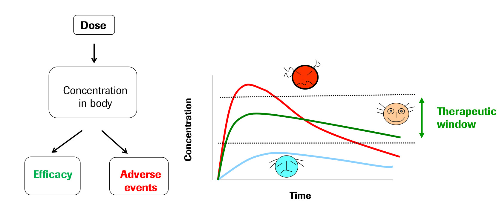
The field of Pharmacokinetics (PK) provides a quantitative basis for describing the delivery of a drug to a patient, the diffusion of that drug through the plasma/body tissue, and the subsequent clearance of the drug from the patient’s system. PK is used to ensure that there is sufficient concentration of the drug to maintain the required efficacy of the drug, while ensuring that the concentration levels remain below the toxic threshold. Pharmacokinetic (PK) models are often combined with Pharmacodynamic (PD) models, which model the positive effects of the drug, such as the binding of a drug to the biological target, and/or undesirable side effects, to form a full PKPD model of the drug-body interaction. This example will only focus on PK, neglecting the interaction with a PD model.

PK enables the following processes to be quantified:

• Absorption
• Distribution
• Metabolism
• Excretion

These are often referred to as ADME, and taken together describe the drug concentration in the body when medicine is prescribed. These ADME processes are typically described by zeroth-order or first-order rate reactions modelling the dynamics of the quantity of drug $q$, with a given rate parameter $k$, for example:

\[ \frac{dq}{dt} = -k^*, \]

\[ \frac{dq}{dt} = -k q. \]

The body itself is modelled as one or more compartments, each of which is defined as a kinetically homogeneous unit (these compartments do not relate to specific organs in the body, unlike Physiologically based pharmacokinetic, PBPK, modeling). There is typically a main central compartment into which the drug is administered and from which the drug is excreted from the body, combined with zero or more peripheral compartments to which the drug can be distributed to/from the central compartment (See Fig 2). Each peripheral compartment is only connected to the central compartment.

The following example PK model describes the two-compartment model shown diagrammatically in the figure above. The time-dependent variables to be solved are the drug quantity in the central and peripheral compartments, $q_c$ and $q_{p1}$ (units: [ng]) respectively.

\[ \frac{dq_c}{dt} = \text{Dose}(t) - \frac{q_c}{V_c} CL - Q_{p1} \left ( \frac{q_c}{V_c} - \frac{q_{p1}}{V_{p1}} \right ), \]

\[ \frac{dq_{p1}}{dt} = Q_{p1} \left ( \frac{q_c}{V_c} - \frac{q_{p1}}{V_{p1}} \right ). \]

This model describes an intravenous bolus dosing protocol, with a linear clearance from the central compartment (non-linear clearance processes are also possible, but not considered here). The dose function $\text{Dose}(t)$ will consist of instantaneous doses of $X$ ng of the drug at one or more time points. The other input parameters to the model are:

• \(V_c\) [mL], the volume of the central compartment
• \(V_{p1}\) [mL], the volume of the first peripheral compartment
• \(CL\) [mL/h], the clearance/elimination rate from the central compartment
• \(Q_{p1}\) [mL/h], the transition rate between central compartment and peripheral compartment 1

We will solve this system of ODEs using the Diffsol crate. Rather than trying to write down the dose function as a smooth mathematical function, we will treat each bolus dose as a discrete event. We first do this procedurally by stopping the solver at each dose time in Rust, then rewrite the same model declaratively using DiffSL stop and reset tensors.

First lets write down the equations in the standard form of a first order ODE system:

\[ \frac{d\mathbf{y}}{dt} = \mathbf{f}(\mathbf{y}, t) \]

where

\[ \mathbf{y} = \begin{bmatrix} q_c \\ q_{p1} \end{bmatrix} \]

and

\[ \mathbf{f}(\mathbf{y}, t) = \begin{bmatrix} - \frac{q_c}{V_c} CL - Q_{p1} \left ( \frac{q_c}{V_c} - \frac{q_{p1}}{V_{p1}} \right ) \\ Q_{p1} \left ( \frac{q_c}{V_c} - \frac{q_{p1}}{V_{p1}} \right ) \end{bmatrix} \]

We will also need to specify the initial conditions for the system:

\[ \mathbf{y}(0) = \begin{bmatrix} 0 \\ 0 \end{bmatrix} \]

For the dose function, we will specify a dose of 1000 ng at regular intervals of 6 hours. We will also specify the other parameters of the model:

\[ V_c = 1000 \text{ mL}, \quad V_{p1} = 1000 \text{ mL}, \quad CL = 100 \text{ mL/h}, \quad Q_{p1} = 50 \text{ mL/h} \]

Procedural approach

To implement the discrete dose events procedurally, we set a stop time for the simulation at each dose event using the OdeSolverMethod::set_stop_time method. During time-stepping we can check the return value of the OdeSolverMethod::step method to see if the solver has reached the stop time. If it has, we apply the dose directly to the state and continue the simulation.

use diffsol::{CraneliftJitModule, OdeBuilder, OdeSolverMethod, OdeSolverStopReason};
use plotly::{common::Mode, layout::Axis, layout::Layout, Plot, Scatter};
use std::fs;
type M = diffsol::NalgebraMat<f64>;
type CG = CraneliftJitModule;
type LS = diffsol::NalgebraLU<f64>;

fn main() {
    let problem = OdeBuilder::<M>::new()
        .build_from_diffsl::<CG>(
            "
        Vc { 1000.0 } Vp1 { 1000.0 } CL { 100.0 } Qp1 { 50.0 }
        u_i {
            centralamount = 0,
            peripheralamount = 0,
        }
        F_i {
            - centralamount / Vc * CL - Qp1 * (centralamount / Vc - peripheralamount / Vp1),
            Qp1 * (centralamount / Vc - peripheralamount / Vp1),
        }
    ",
        )
        .unwrap();
    let mut solver = problem.bdf::<LS>().unwrap();
    let doses = vec![(0.0, 1000.0), (6.0, 1000.0), (12.0, 1000.0), (18.0, 1000.0)];

    let mut central_amount = Vec::new();
    let mut peripheral_amount = Vec::new();
    let mut time = Vec::new();

    // apply the first dose and save the initial state
    solver.state_mut().y[0] = doses[0].1;
    central_amount.push(solver.state().y[0]);
    peripheral_amount.push(solver.state().y[1]);
    time.push(0.0);

    // solve and apply the remaining doses
    for (t, dose) in doses.into_iter().skip(1) {
        solver.set_stop_time(t).unwrap();
        loop {
            let ret = solver.step();
            central_amount.push(solver.state().y[0]);
            peripheral_amount.push(solver.state().y[1]);
            time.push(solver.state().t);
            match ret {
                Ok(OdeSolverStopReason::InternalTimestep) => continue,
                Ok(OdeSolverStopReason::TstopReached) => break,
                _ => panic!("unexpected solver error"),
            }
        }
        solver.state_mut().y[0] += dose;
    }
    let mut plot = Plot::new();
    let central_amount = Scatter::new(time.clone(), central_amount)
        .mode(Mode::Lines)
        .name("central_amount");
    let peripheral_amount = Scatter::new(time, peripheral_amount)
        .mode(Mode::Lines)
        .name("peripheral_amount");
    plot.add_trace(central_amount);
    plot.add_trace(peripheral_amount);

    let layout = Layout::new()
        .x_axis(Axis::new().title("t [h]"))
        .y_axis(Axis::new().title("amount [ng]"));
    plot.set_layout(layout);
    let plot_html = plot.to_inline_html(Some("drug-delivery"));
    fs::write("../src/primer/images/drug-delivery.html", plot_html).expect("Unable to write file");
}

Declarative approach

The same dosing schedule can also be encoded directly in DiffSL. Here the initial condition includes the first dose at \(t=0\), the stop tensor contains the later dosing times \(t = 6\), \(12\), and \(18\) hours, and the reset tensor adds the bolus amount to the central compartment whenever any of those stop conditions fires.

Because the model supplies both stop and reset, the high-level solve method now applies each declarative dose automatically and continues through the full 24 hour simulation.

use diffsol::{CraneliftJitModule, MatrixCommon, OdeBuilder, OdeSolverMethod};
use plotly::{common::Mode, layout::Axis, layout::Layout, Plot, Scatter};
use std::{fs, path::PathBuf};

type M = diffsol::NalgebraMat<f64>;
type CG = CraneliftJitModule;
type LS = diffsol::NalgebraLU<f64>;

fn main() {
    let model = "
        Vc { 1000.0 } Vp1 { 1000.0 } CL { 100.0 } Qp1 { 50.0 } dose { 1000.0 }
        u_i {
            qc = dose,
            qp1 = 0,
        }
        F_i {
            -qc / Vc * CL - Qp1 * (qc / Vc - qp1 / Vp1),
            Qp1 * (qc / Vc - qp1 / Vp1),
        }
        stop_i {
            t - 6.0,
            t - 12.0,
            t - 18.0,
        }
        reset_i {
            qc + dose,
            qp1,
        }
    ";
    let problem = OdeBuilder::<M>::new()
        .build_from_diffsl::<CG>(model)
        .unwrap();
    let mut solver = problem.bdf::<LS>().unwrap();

    let final_time = 24.0;
    let (ys, time, _stop_reason) = solver.solve(final_time).unwrap();
    let q_c: Vec<_> = ys.inner().row(0).into_iter().copied().collect();
    let q_p1: Vec<_> = ys.inner().row(1).into_iter().copied().collect();

    let mut plot = Plot::new();
    plot.add_trace(
        Scatter::new(time.clone(), q_c)
            .mode(Mode::Lines)
            .name("q_c"),
    );
    plot.add_trace(Scatter::new(time, q_p1).mode(Mode::Lines).name("q_p1"));
    plot.set_layout(
        Layout::new()
            .x_axis(Axis::new().title("t [h]"))
            .y_axis(Axis::new().title("amount [ng]")),
    );

    let output_path = PathBuf::from(env!("CARGO_MANIFEST_DIR"))
        .join("../../book/src/primer/images/drug-delivery-declarative.html");
    let plot_html = plot.to_inline_html(Some("drug-delivery-declarative"));
    fs::write(output_path, plot_html).expect("Unable to write file");
}

Adjoints through declarative dose events

The automatic reset handling provided by the declarative approach is useful when the reset itself depends on an input parameter. In the drug-delivery model, we can make the bolus dose an input parameter by putting dose in the DiffSL in tensor. The initial condition uses the same dose for the dose at \(t=0\), and the reset tensor adds dose to the central compartment at later dosing times.

In this example we will integrate the output of the central-compartment concentration squared, \(AUC2 = \int_0^{24} (q_c / V_c)^2 dt\), and then use diffsol’s adjoint capabilities to calculate the gradient of this integral with respect to the dose parameter. The integral of the squared concentration would not typically be of interest, but this example is slightly contrived so that the final gradient is not constant and the plots are non-trivial.

We solve the model forwards in time using checkpointing and extract AUC2 from the final solution, and then create the adjoint equations using the checkpoints and integrate backwards in time to the starting time point. The gradient of AUC2 with respect to dose is then extracted from sg on the final solver state. Repeating this for several dose levels gives the dose-response curve and its gradient.

DiffSL currently needs the LLVM backend for sensitivity-aware reset/root operators in this example.

use diffsol::{
    AdjointOdeSolverMethod, DenseMatrix, LlvmModule, MatrixCommon, OdeBuilder, OdeEquations,
    OdeSolverMethod, OdeSolverState, Op, Vector,
};
use plotly::{common::AxisSide, common::Mode, layout::Axis, layout::Layout, Plot, Scatter};
use std::{fs, path::PathBuf};

type M = diffsol::NalgebraMat<f64>;
type V = diffsol::NalgebraVec<f64>;
type CG = LlvmModule;
type LS = diffsol::NalgebraLU<f64>;

pub fn main() {
    let model = r#"
        in_i { dose = 1000.0 }
        Vc { 1000.0 } Vp1 { 1000.0 } CL { 100.0 } Qp1 { 50.0 }
        u_i {
            qc = dose,
            qp1 = 0,
        }
        F_i {
            -qc / Vc * CL - Qp1 * (qc / Vc - qp1 / Vp1),
            Qp1 * (qc / Vc - qp1 / Vp1),
        }
        stop_i {
            t - 6.0,
            t - 12.0,
            t - 18.0,
        }
        reset_i {
            qc + dose,
            qp1,
        }
        out_i {
            pow(qc / Vc, 2),
        }
    "#;

    let final_time = 24.0;
    let dose_levels = (0..=12)
        .map(|i| 250.0 + f64::from(i) * 125.0)
        .collect::<Vec<_>>();

    let mut problem = OdeBuilder::<M>::new()
        .p([dose_levels[0]])
        .sens_atol([1e-8])
        .sens_rtol(1e-8)
        .out_atol([1e-8])
        .out_rtol(1e-8)
        .integrate_out(true)
        .build_from_diffsl::<CG>(model)
        .unwrap();

    let mut aucs = Vec::with_capacity(dose_levels.len());
    let mut auc_grads = Vec::with_capacity(dose_levels.len());

    for &dose in &dose_levels {
        let ctx = *problem.eqn().context();
        problem.eqn_mut().set_params(&V::from_vec(vec![dose], ctx));

        let mut solver = problem.bdf::<LS>().unwrap();
        let (checkpoints, integrated_output, _output_times, _stop_reason) =
            solver.solve_with_checkpointing(final_time, None).unwrap();
        let auc = integrated_output.get_index(0, integrated_output.ncols() - 1);

        let adjoint_solver = problem
            .bdf_solver_adjoint::<LS, _>(checkpoints, Some(solver), None)
            .unwrap();
        let (adjoint_state, _) = adjoint_solver
            .solve_adjoint_backwards_pass(&[], &[])
            .unwrap();

        aucs.push(auc);
        auc_grads.push(adjoint_state.as_ref().sg[0].get_index(0));
    }

    let mut plot = Plot::new();
    plot.add_trace(
        Scatter::new(dose_levels.clone(), aucs)
            .mode(Mode::LinesMarkers)
            .name("AUC2"),
    );
    plot.add_trace(
        Scatter::new(dose_levels, auc_grads)
            .mode(Mode::LinesMarkers)
            .name("dAUC2/ddose")
            .y_axis("y2"),
    );
    plot.set_layout(
        Layout::new()
            .x_axis(Axis::new().title("dose [ng]"))
            .y_axis(Axis::new().title("AUC2 [ng^2 h / mL^2]"))
            .y_axis2(
                Axis::new()
                    .title("dAUC2/ddose [ng h / mL^2]")
                    .overlaying("y")
                    .side(AxisSide::Right)
                    .position(1.0),
            ),
    );

    let output_path = PathBuf::from(env!("CARGO_MANIFEST_DIR"))
        .join("../../book/src/primer/images/drug-delivery-dose-sensitivity.html");
    let plot_html = plot.to_inline_html(Some("drug-delivery-dose-sensitivity"));
    fs::write(output_path, plot_html).expect("Unable to write file");
}